Introduction

This page contains a brief introduction to the SMS software, for more information please see the Aquaveo Wesite, SMS wiki or the AQUAVEO Learning Center.

There are three versions of SMS available:

SMS Community Edition: A free version suitable for result viewing.
SMS Riverine Pro Version: A paid licence version suitable for advanced TUFLOW result viewing and analysis.
SMS Riverine Pro Version + TUFLOW Interface : A paid licence version. It is a complete modelling package. It is suitable for building TUFLOW models within SMS and the advanced veiewing and analysis of TUFLOW results (paid licence).

Viewing Results

To view results in SMS we need at least two files open. The first is the TUFLOW mesh, this contains information on the location, cells and elevations within the model. The 2D mesh is created by TUFLOW and is outputted with the .2dm extension. A mesh is created for every TUFLOW simulation and has the same name as the TUFLOW simulation. For example if the simulation control file is named M01_5m_003.tcf the TUFLOW mesh will be a file called M01_5m_003.2dm.

Once the mesh has been loaded, the TUFLOW results can be loaded. TUFLOW results can outputted in either the .dat format (1 results file format per output type) or in recent versions of TUFLOW the .xmdf (one output file that contains all of the results).

TUFLOW also writes out a .sup file which contains instructions for SMS to open the 2D mesh first and then the TUFLOW results.

Open the results, by either opening the .2dm and the results files or by opening the .sup file.

Scalar Data

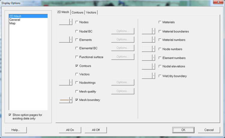
Once you have results loaded into SMS, open the Display Options Dialogue, in the menu items select Display >> Display Options....
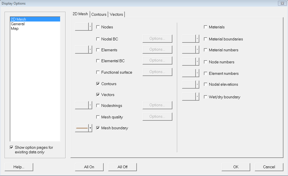
TIP: The shortcut key to bring up the Display Options dialogue is Control + D. In the Display Options dialogue, ensure that you are in the 2D Mesh module in the pane to the left. In the 2D mesh tab, you get a list of options ticking the check box will make an item visible. To see just the scalar results, turn everything off, except Contours.

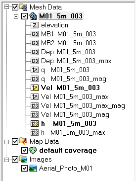
In the project window under Mesh Data is a list of the scalar and vector datasets available.

Scalar datasets are indicated by the icon 123 and vector datasets have 2 arrows as the icon. In the image is the full list of datasets for the TUFLOW tutorial model (Module 1).

A number of datasets appear twice, for example Vel M01_5m_003 is available for viewing as a scalar dataset or a vector dataset (see next section).

An _max in the dataset name indicates that this in maximums throughout the simulation. Dep M01_5m_003 contains the time varying data and Dep M01_5m_003_max contains the peak depths.

Select the scalar dataset that you wish to view.

In the "Time Steps" window, select a timestep and use the up and down arrows to step through the results.

Contouring Options

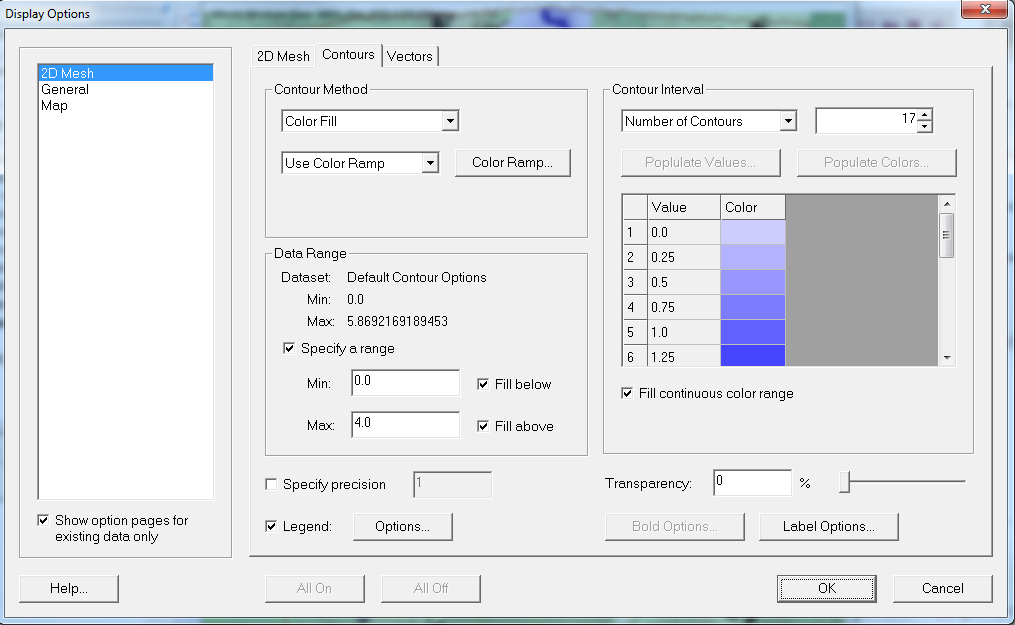
There are numerous options for controlling how the scalar results display (colour profile, contour increment, transparency). This is controlled in the Contour tab in the Display Options dialogue. A brief guide is given below, users are encouraged to experiment.

Bring up the Display Options dialogue, and select the "Contour" tab under 2D Mesh.

Under Contour Method select Color Fill.

TIP:Normal Linear can be used to display contour lines only, and Color and Linear displays both contour shading and contour lines.

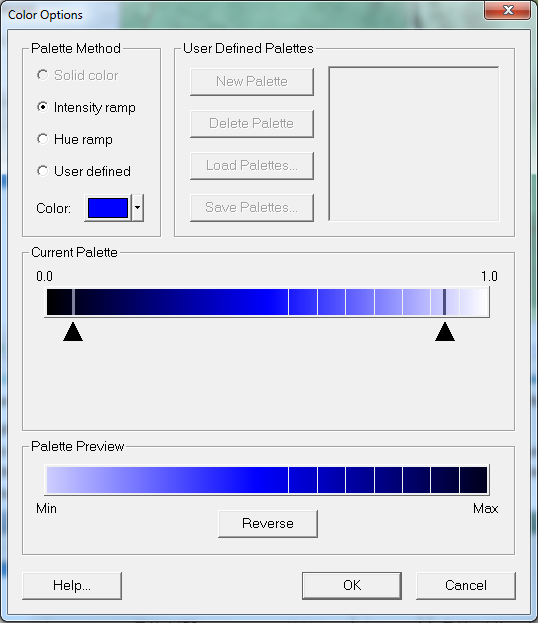
Under "Color Ramp" you can choose the colour profile. There are numerous options here, feel free to experiment. I have chosen an Intensity Ramp varying from light blue to dark blue.

In the Data Range section of the Display Options dialogue there is a summary of the minimum and maximum data values for the selected dataset. A range can specified here, by checking the "Specify a range" option. In the image below an upper range of 4.0 metres, anything above this depth will display in the upper contour range (dark blue).
TIP: by specifying a range and un-checking "Fill Above" or "Fill Below" you can restrict the display range. For example, setting a minimum of 0.1m and un-checking "Fill Below" any depths less than 0.1m will not be displayed.

A transparency can also be set in this dialogue, this can be used to make aerial photos visible beneath the contouring.

Vectors

To turn on the vectors, navigate to the 2D Mesh tab of the Display Options (Display >> Display Options). Check the Vector item, as per the image below.

Select the desired vector item in the project window, scroll through the time steps to view the vectors at each output time.

Vector Display Options

There are numerous option for controlling the size, shape and density of the vectors displayed. This page gives only a brief introduction, users are encouraged to experiment!
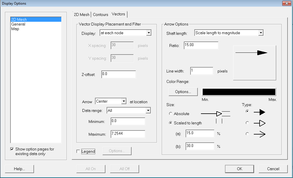
To open the vector options, navigate to the Display Options, select the 2D Mesh in the left hand pane, and then select the Vectors tab, as shown in the image below.

In this dialogue you can control:

If the vectors are shown at each cell corner (Display: at each node) or on a regular grid (Display: on a grid).
Vertical offset (Z offset)

Tip a value of greater than 0 ensures the vectors appear on top of the contours.

The data range (use this to restrict values)
Arrow size, this can be fixed length or scale length to magnitude

Tip scale length to magnitude is recommended for most result viewing

Line width
Colour
Arrow head

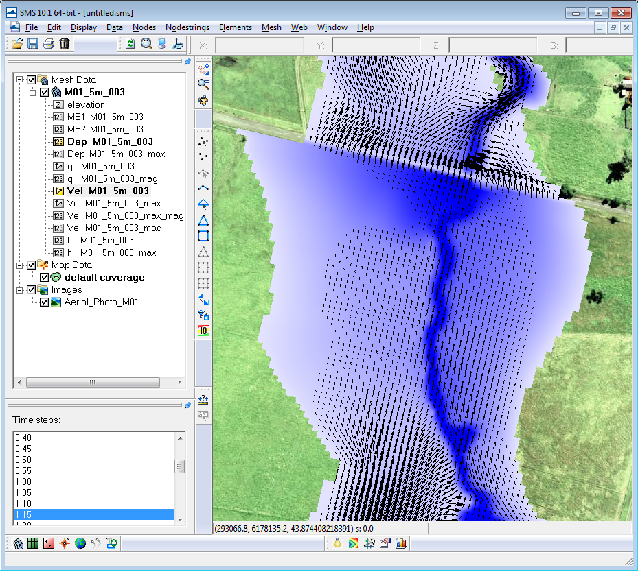
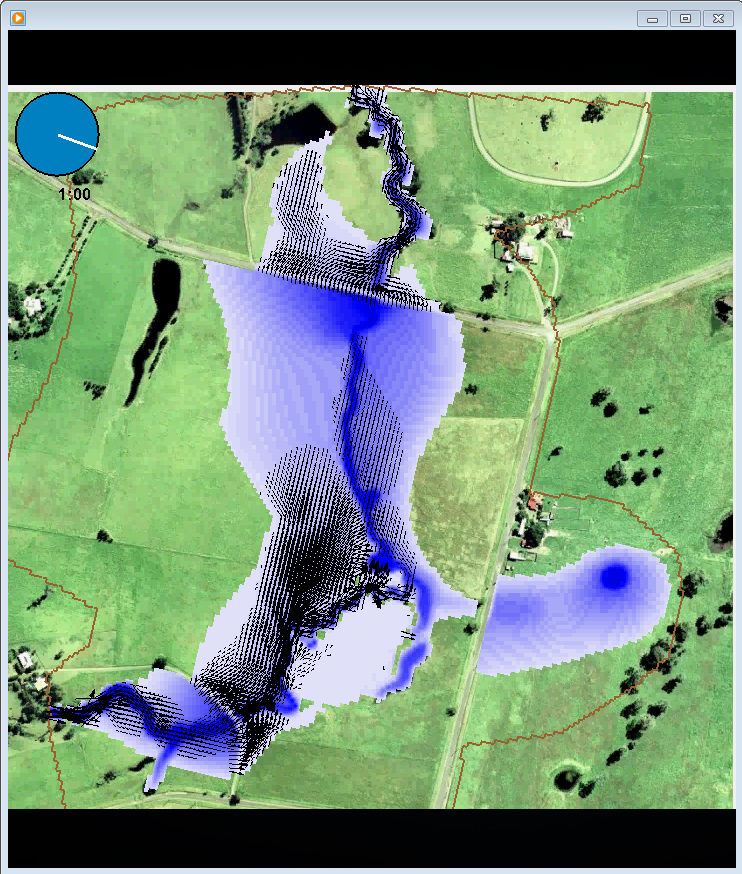
The image below shows velocity vector results displayed with scalar depth results for module 1 of the tutorial model.

Depth and Velocity at time 1:15

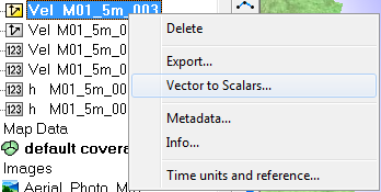
The magnitude for vector results are also available to view as a scalar dataset. Vector results can be converted into scalar results (either Magnitude and direction or X component and Y component). To do this right click on the vector data set in the project window and select Vector to Scalar (as per the image below).

Oblique Views (3D)

SMS is capable of generating animations using oblique map views to simulate a 3D animation. Step by step instructions for creating a 3D animation are available at the SMS 3D Animation page.

Animations

To create an animation in SMS, firstly select the desired (temporal data not maximums), set the display options (for vectors and scalars). Chose an appropriate zoom and window extent.
TIP: to ensure that the colouring and vector magnitudes are appropriate for the entire simulation, it is often beneficial to chose the maximum results dataset when setting.

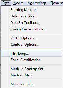
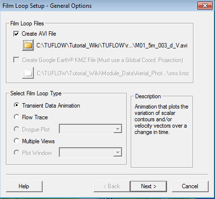
Once you have chosen appropriate display settings ensure that you are in the mesh module, select Data >> Film Loop...'.

Specify a output file name and location in the Film Loop Files section.

Select the Transient Data Animation in the film loop type (default) and select Next.

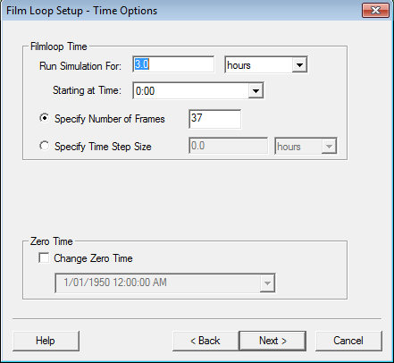
In the next dialogue the time controls can be altered, the default it to create an animation with one output frame per output over the entire event. This can be restricted, for example if nothing exciting happens for the first two hours, you may wish to omit this from the animation. Select next.

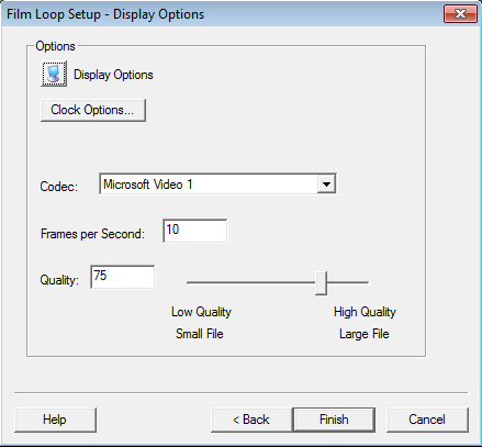
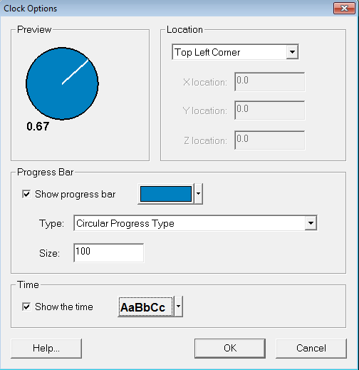
At the next dialogue , we can review and modify our display options, as the changes can;t be seen until the animation starts, it is much easier to do this prior to starting the animation. A clock can also be added.
The output quality and frames per second can be modified here. Once happy with these options select Finish to begin the animation creation.

After a few seconds (or minutes) depending on the size of the results files, an animation should appear. This animation has an .avi extension and should be playable in most media players. Below is a screen grab of the animation in Windows Media Player.