2D Structure Modelling Theory

These webinars by Bill Syme and Greg Collecutt (the TUFLOW Developers) discus the theory behind the energy losses and affluxes modelling associated with hydraulic structures.

2D Bridge Modelling in TUFLOW - Overview

The TUFLOW 2D solution explicitly predicts the majority of “macro” losses due to the expansion and contraction of water through a constriction, or around a bend, provided the resolution of the grid is sufficiently fine (Barton, 2001; Syme, 2001; Ryan, 2013). Where the 2D model is not of fine enough resolution to simulate the “micro” losses (e.g. from bridge piers, vena contracta, losses in the vertical (3rd) dimension), additional form loss coefficients and/or modifications to the cells widths and flow height need to be added.

Contraction/Expansion Losses (“Macro” Losses)

Loss of energy is caused by the flow contraction during the expansion of water after the vena-contracta inside a bridge section and the flow expansion downstream a bridge. As discussed above, this type of "macro" losses can be explicitly resolved by the TUFLOW 2D solver, provided that a proper turbulence model and mesh size are used. Below is an example of the 2D modelling of flow contraction/expansion at a pair of bridge abutments.

Pier Losses

Piers are usually smaller than the 2D cell size in real-world flood models. Although flexible mesh solver or quadtree refinement can be applied to reduce the local cell size around the pier, it also comes with an expensive computational cost that could significantly increase the simulation time. More practically, the backwater effect of piers can be modelled as sub-grid form losses.

Pier form loss coefficients can be derived from information in publications such as Hydraulics of Bridge Waterways (Bradly, 1978) or Guide to Bridge Technology Part 8: Hydraulic Design of Waterway Structures (AUSTROADS, 2019). Energy loss estimated from bridge piers or other obstructions, vertical or horizontal, that do not cause upstream controlled flow regimes like pressure flow, are dependent on the ratio of the obstruction's area perpendicular to the flow direction to the gross flow area of the bridge opening, the shape of the piers or obstruction, and the angularity of the piers/obstruction to the flow direction. For example, using Hydraulics of Bridge Waterways (Bradly, 1978) the approach is:

Calculate the ratio of the water area occupied by piers to the gross water area of the constriction (both based on the normal water surface) and the angularity of the piers. These inputs are used to calculate "J" in the FHA documentation.
Use the Figure 7 Incremental Backwater Coefficient for Piers data to calculate Kp.

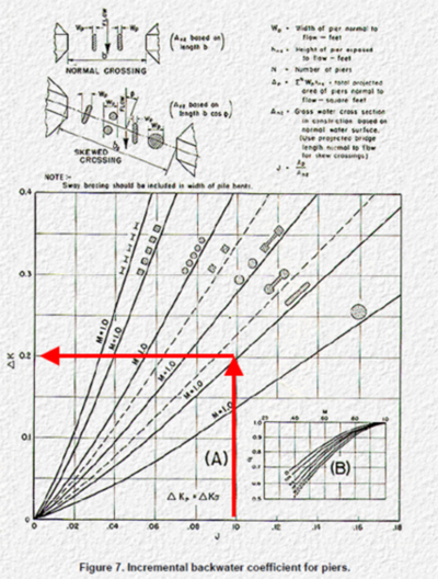
NOTE: the pier form loss coefficients in Hydraulics of Bridge Waterways are derived based on the cross-sectional averaged velocity through the bridge opening in the absence of piers. It's not necessary to specify a blockage value if a pier form loss coefficient estimated from this method is used.

Bridge Deck and Rail (Super Structure)

When a bridge deck become partially or completely submerged, the deck could generate extra afflux resulting in increased water levels and flood extents upstream of the structure. The flow around the deck is highly 3-dimentional and complexed due to the different deck designs/profiles and/or the occurrence of pressure flow. In 2D SWE solver, depth-varying form loss values are often needed to reproduce the afflux caused by such structure. Due to the complexity of the flow, guidelines on how to set the form loss coefficient for the bridge deck are rare. We have carried out a joint research with QLD TMR (Queensland Department of Transport and Main Roads) regarding how to choose a proper form loss value for the bridge deck (Collecutt et al, 2022). In the research, CFD modelling was conducted to investigate the characteristics of energy loss of a simple bridge with a flat bottomed deck and guardrails.

Below are the key findings from the study:

The results displayed a characteristic shape for head loss coefficient as a function of downstream water level over the deck thickness (TW/T).
The head loss (afflux) peaks when the water level is approximately 1.6*T above the bridge soffit, and decays slowly as the bridge becomes progressively drowned out.

The peak loss coefficient value is a function of the ratio of the depth underneath the deck (hB) and the thickness of the deck (T)

Deck Height to Thickness Ratio	Peak Form Loss Coefficient
Scenario A (hB/T) = 2	0.42
Scenario B (hB/T) = 4	0.28
Scenario C (hB/T) = 6	0.20

This table can be used to estimate the deck form loss coefficient based on the bridge design (hB/T). The solid portion of the guard rails (blockage * rail depth) can be added to T in addition to the deck thickness to calculate hB/T. For bridge with more complicated designs (e.g. girders), higher form loss might be required due to the higher surface roughness of the bridge.

NOTE: This form loss value should not be confused with the value of 1.56 used in the pressure flow approached adopted in TUFLOW 1D "B" and "BB" bridge. TUFLOW 1D bridge pressure flow approach is based on the section 4.13.2 "All Girders in Contact with Flow (Case II)" of Guide to Bridge Technology Part 8: Hydraulic Design of Waterway Structures (AUSTROADS, 2019). The original hydraulic experiment conducted by Liu et al (1957) in a laboratory flume with a pair of bridge abutments and a deck. The flow conditions were similar to orifice flow due to the high blockage ratio caused by the abutments and the deck. When modelling bridges in 2D, the contraction/expansion losses caused by the abutments would be handled explicitly by the 2D solver, so a value 1.56 can lead to duplication of the contraction/expansion losses caused by the bridge abutments.

TUFLOW 2D Bridge Setup

Traditionally, 2D Layered Flow Constriction (2d_lfcsh) has been used in TUFLOW 2D modelling to specify the depth varying form loss of a bridge structure. As of 2022 release a new GIS layer called 2D BG Shape (2d_bg) has been implemented in order to simplify the model input based on the findings from the joint TMR study. Both methods provide options for representing flow surcharging, the pressure flow of bridge decks and eventually submerged bridge flow at higher water levels. During the surcharging of bridge decks, higher energy losses can be specified to simulate the pressure flow. Four flow constriction layers are represented. The lower three layers represents the pier, the bridge deck and the rails. Each layer has its own attributes to specify the blockage and the form loss coefficient. The top (fourth) layer assumes the flow is unimpeded, representative of flow over the top of a bridge. Within the same shape, the invert of the bed, and thickness of each layer can vary in 3D.

2D Layered Flow Constriction (2d_lfcsh)

Four layers are used for 2d_lfsch:

Layer 1: Beneath the bridge deck. If bridge piers exist a small form loss is usually expected due to the energy losses associated with the piers. Hydraulics of Bridge Waterways (Bradly, 1978) can be used to estimate the pier form loss coefficient.
Layer 2: The bridge deck. This would be 100% blocked and the form loss coefficient would increase due to the additional energy losses associated with flow surcharging the deck. The hB/T vs FLC table from the joint research with TMR can be used to estimate the deck form loss coefficient.
Layer 3: The bridge rails. These might be anything from 100% blocked (solid concrete rails) to 10% blocked (very open rails). Sensitivity testing with 100% blockage is recommended as often debris during a flood can be substantial (see images from the Q&A section below). Some form losses would be specified depending on the type of rails and blockage. The solid portion of the rails (pBlockage*L3_Depth) can be added to L2_Depth to calculate hB/T in the table above to estimate the combined form loss coefficient of the L2 and L3.
Layer 4: Flow over the top of the rails - flow is assumed to be unimpeded.

The 2d_lfcsh functions by adjusting the flow width and the form loss of 2D cell faces. The combined blockage across the 4 layers is calculated at each simulation timesteps:

_i

i

_total

The combined form loss coefficient can be estimated using different approaches, which can be individually specified by the 2d_lfcsh Shape_Options attribute, or globally specified by command:
Layered FLC Default Approach == [ CUMULATE | {PORTION} | METHOD C ]

CUMULATE (Method A): the losses are accumulated as the water level rises through the layers according to the following equation.

PORTION (Method B): the losses are applied pro-rata according to the depth of water in each layer using the equation below.

METHOD C: this approach combines the CUMULATE and PORTION approaches by utilising CUMULATE through to the top of Layer 3 and PORTION above Layer 3.

All three methods apply a constant form loss value of L1_FLC when the water level is below Layer 2. Above Layer 2, the total form loss coefficient is increased gradually based on the thickness of water in Layer 2 and 3. Due to the depth proportioning approach used in the PORTION approach, larger L2_FLC/L3_FLC values are needed to achieve the same peak form loss coefficient as the other 2 methods. Above Layer 3, the PORTION and METHOD C approaches gradually reduce the total FLC with the increase of the water level, while the CUMULATE method continues to applies the cumulated form loss value. An example, taken from a calibration of a bridge structure from the Iowa River Flood Study is shown below. With water slightly overtopping a bridge deck, a combined form loss coefficient of 0.35 was used to match the observed head loss.

Layer	Depth (m)	Blockage (%)	Form Loss Approach
Layer	Depth (m)	Blockage (%)	CUMULATE	PORTION	METHOD C
1	5.0	5	0.07	0.07	0.07
2	1.5	100	0.15	1.05	0.15
3	1.0	50	0.13	0.70	0.13

The figure below compares how the form loss value varies with height for the 3 methods.

2D BG Shape (2d_bg)

2D BG Shape is similar to the Layered Flow Constriction, but has several update to simplify the input based on the findings from the joint study with TMR. The lower three layers have been renamed for clarity.

Pier layer: Similar to Layer 1 in Layered Flow Constriction.
Deck layer: The bridge deck.
Rail layer: The bridge rails. The deck layer and the rail layer are treated as one Super Structure layer in 2d_bg. A combined form loss coefficient is specified using the 'SuperS_FLC' attribute. The solid portion of the rails (Rail_pBlockage*Rail_Depth) is added to Deck_Depth to calculate hB/T in the table above to estimate the combined form loss coefficient of the Super Structure.

Layer 4: Above the top of the rails, flow is assumed to be unimpeded.

Inflection Point: As shown in the joint study above, the head loss peaks when the water level is approximately 1.6*T above the bridge soffit, and decays slowly as the bridge becomes progressively drowned out. The 'SuperS_IPf' attribute (inflection point factor, default = 1.6) can be used to define the height of the inflection point. The solid portion of the rail layer is also added to the deck thickness to calculate the depth to the inflection point (D_IP), i.e.:

The form loss approach is similar to the FLC approach METHOD C, with L2/L3 replaced by a single super structure layer:

Using the same bridge example with SuperS_FLC of 0.28 and SuperS_IPf of 1.6, D_IP would be set as 3.2m above the bridge soffit, and the figure further below shows how the form loss value varies with height.

Layer	Depth (m)	Blockage (%)	Form Loss
Pier	5.0	5	0.07
Deck	1.5	100	0.28
Rail	1.0	50	-

2D Bridges Line vs Polygon Layer

The form loss coefficient (FLC) is applied differently when using a line compared to a polygon. The FLC is applied at cell sides (u and v faces) as this is where velocities are calculated.
When using a polyline, the FLC attribute depends on the type of the polyline:

Thin line (width attribute of zero) - The FLC attribute in the GIS object should reflect the total form loss value for the bridge. A thin 2d_lfcsh line will apply the FLC to a single row of cell sides. As such, this approach is cell size independent. Thin line lfcsh are the easiest setup, and is the preferable recommended approach.
Thick line (width attribute between zero and 1.5 times the cell size) - The FLC attribute is half of the total loss as the form loss is applied on each cell side of the selected cells. A cell is selected if the polyline intersects the cell crosshair. Caution should be taken when using a "thick" line, due to the fact changes in cell size can trigger a "thick" line to become a "wide" line. If this were to occur the FLC attribute would need to be recalculated to not overestimate losses.
Wide line (only supported for 2d_lfcsh, width attribute larger than 1.5 times the cell size) - The FLC attribute is a portion of the total loss based on number of cell sides in the predominant direction of flow. Caution should be taken when using a "wide" line due to the fact changes in cell size can trigger the need to recalculate and define losses.

The number of cell sides and the assigned FLC value can be checked in the lfcsh_uvpt_check and bg_uvpt_check files.

For larger bridges that spread across multiple cells, it is recommended to use a polygon layer, which selects all u and v faces falling within the polygon. Caution should be taken when specifying the FLC values for the two different 2d bridge features:

2d_lfcsh: FLC attribute is the total loss per unit length (meters or feet) in the direction of flow. The FLC is applied to each face as 'FLC * cell size'
2d_bg: FLC attribute is still the total form loss. Instead of converting it to "form loss per meter", the "Deck_Width" attribute is used to automatically distribute the total FLC to the selected faces, i.e. FLC_face = FLC / Deck_Width * cell size.

It is a good modelling practice to check the lfcsh_uvpt_check and bg_uvpt_check files to confirm the number of faces selected and the FLC values assigned. It is also strongly recommended to undertake a sensitivity analysis on the applied form losses in the model to check if it makes any difference to the results and/or double check against other methods (hand calculations, other software, CFD modelling), especially if the bridge is anywhere near the area of interest. If calibration data is available, this should be used to guide the form loss value specification.

Common Questions Answered (FAQ)

What blockage values should I use for bridge guard rails?

The blockage of bridge guard rails can be anything from 100% blocked (solid concrete rails) to 10% blocked (very open rails). In addition, the accumulation of debris during a flood can be substantial as shown in the image below. Sensitivity testing with 100% blockage is recommended.

How to conduct sensitivity test for 2D bridges?

General recommendations to cross-check the results are:

Compare computed affluxes against desktop methods (e.g. Hydraulics of Bridge Waterways, 1978) and/or other software including CFD, especially for unusual bridge designs.
Use any recorded flood marks or general observations from past events to check and calibrate FLC values.
Conduct sensitivity testing by assessing the impact and influence of FLC values on your modelling objectives. The afflux resulting from the FLC values will be proportional to the velocity head, i.e. ∆h=FLC*(v^2/2g). As such, if velocities are low (e.g. 1 m/s), the results may not be overly sensitive to uncertainties in the FLC values. If completing a check using this equation for a long skew bridge it is best to calculate the total structure velocity from a PO line digitised in the same location as the bridge.

Finally, after completing sensitivity testing and understanding the range of uncertainty due to unknowns like the degree of blockage and influence of FLC values (e.g. +/-20%), you are in a position to discuss with your client how best to proceed. For example, if the modelling is to set planning levels for a development upstream then it may be appropriate to choose values on the higher side (higher FLC values and/or blockage assumptions), noting that the uncertainty may be amply covered by a regulatory freeboard. Conversely, if the development is on the downstream side the conservative approach would be to use the results at the lower end of your FLC/blockage values.

Should I use both FLC and blockage for layer one in 2D bridge layered flow constriction?

When applying FLC and blockage values to model obstructions such as piers, the following considerations need to be taken into account:

The FLC value applies an energy loss along 1D channels or across 2D cell faces equivalent to FLC*V²/2g where V is the 1D channel velocity or the 2D cell face velocity.
FLC values are often sourced from publications such as Hydraulics of Bridge Waterways or AustRoads (e.g. Kp chart for piers).
If possible, establish whether the source of the FLC value is based on the approach velocity (the velocity in the absence of piers) or structure velocity (the velocity with area blocked out by the piers) noting that it often isn’t clear or stated.
- If it is the structure velocity, this is usually the velocity at the vena-contracta (point of greatest contraction within the entrance to the structure and therefore highest velocity) - see image below. Bluff or sharp-edged obstructions will have a much more pronounced vena-contracta, and therefore higher velocity compared with a round-edged obstruction.
- FLC values based on the approach velocity will be higher than those based on the structure velocity to achieve the same energy loss.
Applying a blockage equivalent to the obstruction width will increase, usually very slightly, the velocity of the 1D channel or 2D cell face. This won’t be the vena-contracta velocity, but a velocity between the approach velocity and the vena-contracta velocity. A greater blockage will need to be applied to emulate the vena-contracta velocity.
If the FLC source value is based on:
- The approach velocity then there is no need to apply a blockage value.
- The structure velocity then the blockage value should be applied noting that it may be appropriate to apply a larger blockage to take into account the vena-contracta.
If it is not clear or unknown whether the FLC source value is based on the approach or structure velocity, the recommendation would be to apply the blockage in the interests of being slightly conservative on the upstream flood level calculation.
For most minor obstructions such as bridge piers, the blockage is usually relatively small and whether included or not has a negligible or minor affect on flood levels compared with other factors such as the approach embankments and the bridge deck.
Blockage from debris wrapped around piers can have a greater influence on the results than the effect of applying or not applying a blockage.
As always, sensitivity testing with and without blockage and +/- the FLC value is highly recommended to understand their importance in regard to the broader modelling objectives and the effects of uncertainties in the input data, boundaries, other parameters such as Manning’s n values, and the accuracy of the numerical solution scheme (see Maximising the Accuracy of Hydraulic Models webinar).

Image showing the formation of the vena-contracta.

I don't see results that I expect when using 2d_lfcsh layer

The 2d_lfcsh layer is a versatile feature that was designed to model bridges in 2D, but can also be used for other applications like fences, buildings raised on pillars and so on. Some of the unexpected results could be:

Water level going through the bridge deck in 2D map output.
Water transiting through 100% blocked Layer 1, e.g. fences with solid base.
SHMax.csv reporting values above the bridge deck when 2D map output reports water level lower than the top of the bridge deck.

TUFLOW is a 2D solution (not 3D), in the 2d_lfcsh layer the percent blockage and form loss coefficient applied to the cell faces is depth averaged across the entire cell face (across Layer 1, 2 and 3):

For bridges, where Layer 2 has a 100% blockage applied, the minimum flow width of 0.001m is used and is averaged with the Layer 1 blockage (based on the depth of the water). This may result in a water level being reported within or above the bridge deck, which would represent the pressure head.
Layered flow constriction works by adjusting the flow area of the cell faces by any blockages to generate the correct depth averaged velocity at each face at which the form losses are applied as a fraction of the V²/2g kinetic energy. Calculating the correct velocity is critical for determining the losses as the losses are proportional to the velocity squared.
For a layered flow constriction cell face the flow area cannot be zero above the invert of Layer 1 to avoid a divide by zero in the computations, therefore a minimum average flow width after applying blockages of 0.001 m is applied. if Layer 1 is 100% blocked, a very small amount of water will flow through Layer 1. If this is unacceptable, instead of applying 100% blockage of Layer 1, the preferred approach is to start the layered flow constriction at the top of Layer 1 or raise the ground elevation to the top of Layer 1 using one of the Z Shape modification functions (e.g. a breakline).

Can I model bridge piers explicitly in 2D using very small cells?

It isn't recommended to explicitly model bridge piers in TUFLOW, or any other 2D or 3D software (the possible exception being CFD software), but the reasons why are a little complicated.

Small scale obstructions to the flow, such as trees, poles, piers, etc. cause additional head losses along a flow path due to their drag characteristics. Historically, drag (or form loss) coefficients for various profile shapes have been determined as a function of Reynold’s number through experimental testing. More recently, computational fluid dynamics (CFD) has been used to attempt to reproduce the velocity field in the wake of such objects, although providing better results than 2D modelling, the results have not always agreed well with physical tests. In particular the drag of a given profile depends on the exact location of flow separation points, which in turn depends on the ability of the CFD code to predict the laminar to turbulent transition in the boundary layer, which is many times smaller than the profile shape itself. In general, the form loss results from CFD models show significant sensitivity to mesh size, mesh design, and choice of turbulence model, therefore, considerable caution needs to be exercised even for CFD modelling.

The point of flow separation around an object has a major bearing on the drag coefficient and is not reliably reproduced by 2D or 3D software.

Modelling 2D flow around profiles with the 2D or layered 3D form of the shallow water equations (SWE) as used by TUFLOW and other free-surface water flow solvers, is no different in this regard. While mesh-resolved wakes behind the piers using a fine mesh can be seen in the results, the predictions for head losses show the same sensitivities (mesh size, mesh design, choice of turbulence model) as seen in 3D CFD.

The safest and strongly recommended approach with regard to establishing head losses and therefore flood levels, is to not resolve the obstructions in the mesh but instead model the effects of such obstructions with form (drag) loss coefficients (applied to selected mesh cells) that have been derived from physical testing. This approach has been shown to provide the most consistent results across various mesh resolutions. It also has the added benefit that, by avoiding small cells in the mesh, it will provide much more efficient run times for flow solvers.

How to best convert flow constriction data (2d_fc or 2d_fcsh) into newer formats (2d_lfcsh or 2d_bg)?

The form loss parameters can be transferred from the flow constriction (2d_fc or 2d_fcsh) to the first layer of the layered flow constriction (2d_lfcsh) or pier layer of the 2d_bg. Definition of the remaining form loss and blockage layer inputs should follow the guidance outlined in 2D Layered Flow Constriction and 2D BG Shape paragraphs.
When using floating pontoon (type FD in the 2d_fc or 2d_fcsh) different setup might need to be used for different events. For large events when floating pontoon becomes fixed at the top of the supporting piles, standard 2d_lfcsh setup can be used. Smaller events when the pontoon is floating at different heights might require more sensitivity testing of the structure parameters to find out a setup the matches the reality as close as possible.

Should I model bridges in 1D or 2D Domain?

The recommended approach typically depends on the study objectives and if the channel upstream and downstream of the bridge is modelled in 1D or 2D. To preserve the momentum as accurately as possible the bridge should be modelled in the same dimension as the channel, e.g. 1d_nwk bridge if the channels is in 1D and 2d_bg or 2d_lfcsh if the channel is modelled in 2D.
In 2D, the expansion/contraction losses are modelled based on the topography and don't need to be estimated as attributes as for 1D modelling. Also, for higher flows where the bridge is overtopped, 2D is preferable approach.

What is the difference between downstream and upstream controlled flow?

Downstream control means a change in downstream water level will cause a change in upstream water level. Upstream control means the upstream water level is insensitive to the downstream water level and usually indicates the occurrence of supercritical flow.

Up
Back to TUFLOW Modelling Guidance

TUFLOW 2D Hydraulic Structures

Contents