FMA Challenge 1 (1D-2D linked)
Introduction
If you haven't already completed the tutorial models, please see this tutorial model page. This page is for TUFLOW users of intermediate to advanced ability.
In this challenge, a fully two-dimensional model with a nested one dimensional model will be developed to explore an Urban Riverine conditions with an urbanized over-bank floodplain. The model includes several hydraulic structures/bridges within the main stream system which will impact flood elevations. Flooding within the urbanized over-bank floodplain is expected.
From this challenge, it is expected the user will develop their skills in:
- Nested 1D/2D models;
- Understanding Urban Riverine conditions and over-bank floodplains,
- Understanding of the influence of hydraulic structures;
- Using scenarios and variables to determine a suitable cell size, timestep and log output scenarios; and
- Using bc layers with HX, XP, CD and CN types altogether.
Data for this model is provided via ZIP compressed file posted on the internet/FTP for download.
Relevant Tutorials
Although all tutorials are directly relevant to the challenges, it may be useful to revisit some of the finer details as follows:
- 1D-2D Linking- Tutorial Module 2
- Running Events and Scenarios- http://www.tuflow.com/forum/index.php?showtopic=1149&hl=scenario
Data Notes
The original data for this analysis has been modified from its original datum and original elevations have been altered and corrupted such that the data would not be usable for real world modeling, analysis and mapping. Datum data has been stripped from the files provided. A combination of statute (ft) and metric (m) data is provided in the challenge data. Analysis may be performed in metric or Statute units, however all returned data shall be delivered to FMA in Statute (ft) units. Additionally, some of the provided data indicates vertical Datums 29 and 88. We have verified all data provided is in the same vertical datum and for this model challenge assume that is the vertical datum “FMA 12”.
Information to Modelers
Assignment of all parameters for this analysis are at the discretion of the modeler. A high resolution aerial image is provided so that land cover details can be inspected. Information on the problem definition can be found on FMA_Challenge_Models/FMA_Scenario1/FMA_Challenge_Model_Introductions.
Relevant Files
It is up to the modeler's discretion to determine what GIS package to use, what text editor to use, and how to run their models (batch mode or within the text editor).All relevant files can be found on FMA_Challenge_Models/FMA_Scenario1/
Solution
A sample solution has been presented, courtesy of BMT WBM.
Cross Section Spacing, Grid Size and Mesh Element Size
The modeling approach represented the in-bank area with 1D elements dynamically linked to a 2D grid domain to represent the overbank floodplain.
The 1D sections provided were used for the in-bank topography. The overbank (2D) areas were modeled using 10ft and 15ft resolutions. The 2D grid dimension (rotated) was 17,500ft by 8,000ft. A total of 87 cross-sections were used for the 1D in-bank domain.
Structures were modeled as a combination of bridges and culverts. For bridges, height varying energy loss tables were used based on the Hydraulics of Bridge Waterways (Bradley, 1978). For culverts, TUFLOW simulates all possible inlet and outlet controlled flow regimes with automatic switching between regimes. The calculations of culvert flow and losses are carried out using techniques from “Hydraulic Charts for the Selection of Highway Culverts” and “Capacity Charts for the Hydraulic Design of Highway Culverts”, together with additional information provided in the literature such as Henderson 1966.
The number of cross sections and mesh elements used are as follows:
| 2D Cell Size | 1D Sections | Active 2D Cells |
|---|---|---|
| 15ft | 50 | 286,434 |
| 10ft | 87 | 643,565 |
Computational Domain Assembly
TUFLOW directly reads GIS data layers to construct models. The layers used/created for Challenge 1 are:
- A DEM TIN created from the provided terrain data (2ft contours) and exported to ESRII ASCII format as a 2ft DEM grid. When TUFLOW reads this DEM it interpolates the elevations onto the 2D computation grid.
- GIS layers of cross-section locations and 1D network including structure details.
- GIS land-use layer digitized in .shp format.
- GIS layer of 1D/2D interface lines along the left and right banks of the channels. All model inputs are independent of the 2D grid cell size, orientation and extent, allowing for different 2D resolutions, dimensions and orientation to be easily simulated. Peak flood depths and water levels were exported to ESRII ASCII grids, and the flood extent was created by contouring the grid into a single region. Flows are outputted in .csv format and directly loaded into Excel. Profiles were created using the post processing utility TUFLOW_to_GIS and outputted into a .csv file.
- The use of contour data to create the DEM; and
- The model boundary/terrain data does not extend beyond the flooded area.
Challenges
The typical challenges experienced in situations similar to this usually relate to:
The presented solutions to these challenges are as follows:
Using Contour Data to Create the DEM
Contour data, without additional point elevations and/or 3D breaklines, is difficult to triangulate or interpolate to create an accurate DEM. The consequence of solely using contours is the resulting DEM can have a terraced or stair-step surface that contains flat sections where the contours form a U shape.
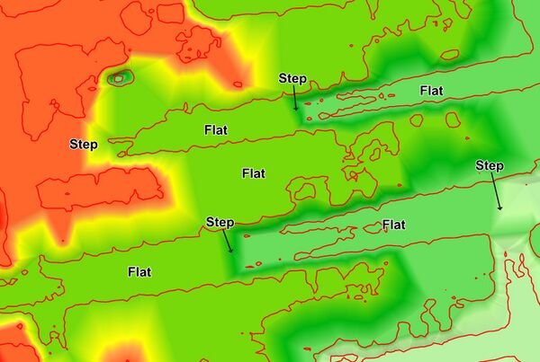
For example, the image below shows a part of the DEM. The red lines are the 2ft contours provided. Where the contours form a U shape, the triangulation or interpolation method typically forms flat (horizontal) areas inside the U as labeled “Flat” in the image. Between the Flats, Steps occur representing the drop in elevation to the next contour level.

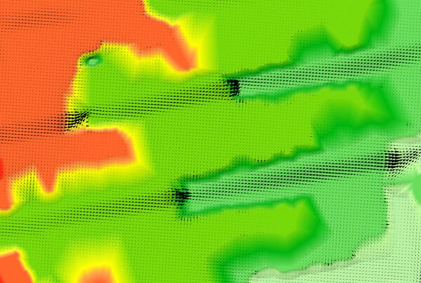
When the 2D flow patterns are observed, as per the velocity arrows in the image below, the water appears to be “cascading” down the roads. Along the flat areas the velocities are low, and where the elevations suddenly drop to the next flat section the velocities are high, thereby creating the cascading effect.

The 2D flow patterns reflect the terraced or stepped nature of the DEM, which is not a realistic representation of the road topography. Some interpolation methods such as IDW (Inverse Distance Weighting) can provide a smoother DEM, but may not preserve the contours, and where the U shapes are pronounced they will still have a strongly terraced effect.
The resulting 2D depths and water levels are also unrealistic as can be seen in the image below. The blue shades are the depths and the blue lines the water level contours every 0.5ft. Where the steps occur in the DEM, the water level contours are closely spaced, and along the flats they are wide apart. The depths vary significantly along the road when they should be reasonably uniform.