Tutorial Module02 Archive
- Save a copy of M01_5m_002.tbc (TUFLOW\model\ directory) as M02_5m_001.tbc.
- Add the following lines to the .tbc file.
For MAPINFO users add:
Read GIS BC == mi\2d_bc_M02_culverts_001.MIF
For ArcGIS or QGIS users add:
Read GIS BC == gis\2d_bc_M02_culv_001_P.SHP
Read GIS BC == gis\2d_bc_M02_culv_001_L.SHP
- Save the file.
- Output Folder == ..\results\M02\1d\
- ...
- Save a copy of the TUFLOW control file M01_5m_002.tcf as M02_5m_001.tcf.
- Add the following lines to the .tcf file:
Start 1D Domain
- Output Folder == ..\results\M02\1d\
- Write Check Files == ..\check\1d\
- Output Interval (s) == 180 ! Output every 3 minutes. Note the (s) is required to output indicate value is in seconds
- Timestep == 0.75 ! Set 1D timestep to be half the 2D timestep
MapInfo Users
- Read GIS Network == ..\model\mi\1d_nwk_M02_culverts_001.mif
- Read GIS Network == ..\model\gis\1d_nwk_M02_culverts_001_L.shp
- Read GIS Network == ..\model\gis\1d_nwk_M02_culverts_001_P.shp
End 1D Domain
- Output Folder == ..\results\M02\1d\
- We need to change the reference to the update .tbc file, otherwise the previous version would be used and the 2D connections in the 2d_bc layer would not be created:
BC Control File == ..\model\M02_5m_001.tbc
- Now that we are running Module 2, we will also update the Output Folder to:
Output Folder == ..\results\M02\2d\
- Save the .tcf file changes.
- In 2D: Write Check Files == ..\check\2d\
- In the 1D block: Write Check Files == ..\check\1d\
- In Windows Explorer navigate to the TUFLOW\results\M02\2d\plot\csv\ folder.
- There should be multiple .csv files in the directory.
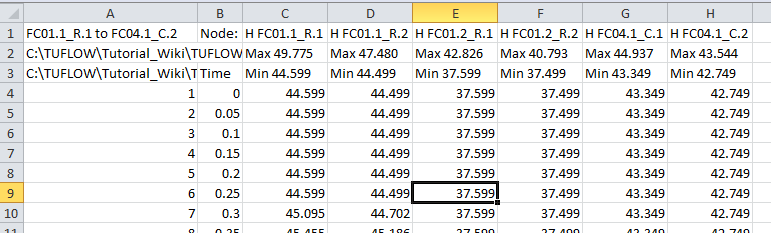
- The M02_5m_001_1d_H.csv, M02_5m_001_1d_V.csv and M02_5m_001_1d_Q.csv files contain the time-series of water level, velocity and flow.
- Open the M02_5m_001_1d_H.csv in Excel by double clicking on the file (this should be the default program for this type of file).
- At each of the nodes (upstream and downstream of each culvert) are the water levels every 3 minutes (set in the .tcf). TUFLOW automatically created nodes at the ends of the culverts. These nodes have the name of the culvert with either .1 (upstream node) or .2 (downstream node) appended. For example FC01.2_R.1 is the node upstream of culvert FC01.2_R.
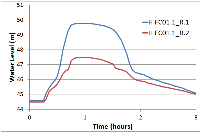
- The standard Excel charting features can be used to graph the results (using the XY scatter chart type). A chart of the water levels upstream and downstream of culvert "FC01.1_R" is shown below.
- Open the _V and _Q .csv files and review the flow and velocity results.
- Other 1D results are also written to the TUFLOW\results\M02\1d folder. The _MB.csv and _MB1D2D.csv contain mass balance information, these files will be introduced in later tutorial modules.
- Save date of .tab file is later than .mif or .mid
- Error 2024 - Could not find a 1D node snapped to CN line
- Error 2028 - Could not find a CN object or 1D node snapped to 2D SX object.
- Why does the TUFLOW DOS Window open, though the TCF isn’t read and the simulation doesn’t execute?
- Save the TUFLOW runfile M02_5m_001.tcf as M02_5m_002.tcf.
- Add the following command to the TCF file:
- Solution Scheme == HPC ! Use the HPC solver to run the model
- Solution Scheme == HPC ! Use the HPC solver to run the model
- If you have a CUDA enabled NVIDIA GPU device, you can also add the following command to run the HPC solver using GPU hardware:
- Hardware == GPU ! Run HPC solver on GPU
- Hardware == GPU ! Run HPC solver on GPU
- Save the TCF file and run the model.
- Check the simulation logs in the DOS window, .tlf and .hpc.tlf log files. What proportion of the compute effort was spent on the 0D (initialisation, input / output communication between CPU and GPU, etc.), 1D modelling (CPU) and the 2D modelling (GPU)? Example compute percentage output is highlight below from the DOS window.
- View the results in your preferred package. How do they compare to the TUFLOW Classic results?
Introduction
A purely 2D model was developed during the Module 1. You may have noticed, when reviewing the results, that some road embankments were causing a damming effect across the main channel. In reality there are culverts beneath these embankments. We will add 1D culverts to the 2D model created in Module 1 in this Module.
The main steps in the process are outlined in the Table of Contents at the top of the page.
The only new file type that is introduced in this module is the 1d_nwk GIS layer. This layer defines the 1D or quasi-2D (branched 1D) domain network of flowpaths (channels) and storage areas (nodes).
Define 1D Structures
There are three culverts that will be modelled in this module. The locations of these structures has been provided in the Module_Date\Module_02\GIS\ folder. To define the 1D network for TUFLOW input, please select your GIS package from the list below:
Define 1D/2D Linkages
We now need to specify how the 1D culverts is linked to the 2D domain. For this tutorial we will use two different methods to highlight the two main approaches to creating the linkage.
The setup of the link is done in your GIS package, please select your chosen GIS package from the list below:
Simulation Control Files Updates
We now need to update our TUFLOW Control File (TCF) to ensure that our GIS layers are read in. We have made no changes to the geometry, or inflows, so we do not need to change the our TUFLOW Geometry Control (TGC) file or boundary condition database (bc_dbase). We have added the 1D/2D links, which need to be defined within the TUFLOW Boundary Control (TBC) file.
TUFLOW Boundary Control File (TBC) Updates
For SMS users, you do not need to modify these files manually, it is automatically done when you export TUFLOW files from SMS. Follow the instructions on page "Export TUFLOW Simulation"
TUFLOW Control File (TCF) Updates
A separate 1D control file, which has the extension .ecf can be used to include the additional commands associated with the 1D model. However, for simple 1D inputs such as this, the 1D commands can be included within the 2D TUFLOW Control File (TCF). For the more complex case of an open channel carved through the 2D model domain (Module 4) a separate 1D ESTRY Control File (ECF) will be used.
There are two ways of including 1D command in the 2D TCF, a 1D prefix can be added for single commands. For example to set the output folder for 1D outputs the following command can be added to the TCF:
1D Output Folder == ..\results\M02\1d\
Alternatively if multiple 1D commands are to be added these can be added within a 1D Domain control block. The control blocks are defined with a start and an end command as per the example below:
Start 1D Domain
End 1D Domain
As this is a simple model, we will use the later method. The commands are dependent on the GIS package.
SMS Users, you do not need to modify these files manually, it is automatically done when you export TUFLOW files from SMS. Follow the instructions on page "Export TUFLOW Simulation"
Run the Simulation
Using your preferred method for starting TUFLOW, run M02_5m_001.tcf. Please refer to Module 1 for a detailed description of the various methods for running a TUFLOW simulation. Example batch files have been included in the complete model download for reference.
Error 2050
The model should have failed to start with "Error 2050" generated as per the image below:

This error indicates that at a "SX" type connection, the lowest ground elevation in the 2D cells is higher than the invert of the culvert. For this connection to work the 2D cell elevation must be below the invert of the culvert.
The reason for this is that the "SX" type boundary is a source boundary for the 2D cells (the source comes from the 1D model), the 1D model has a water level boundary applied from the 2D cells. Even when the 2D cells are dry, the level is above the 1D channel invert and mass could be created. TUFLOW does not allow this to happen and Error 2050 is reported.
To locate the area that where this is occurring, we will load the messages layer into our GIS package, please pick from the list below:
Tip: Remember and get into the habit of using the messages layer, this allows you to quickly locate problems.
Note: In the example above, the cause of the difference in elevations between the 1D culvert and the 2D cells was due to an incorrect invert in the data provided. However, this issue can also occur if the culvert inverts come from accurate ground survey and the elevation in the 2D is based on less accurate (for example LiDAR / ALS) data. If the culvert invert data is of a higher quality the elevations in the 2D cells should be lowered to match the culvert elevation. We will cover 2D topography modifiers (e.g. breaklines) in Module 3.
Re-Run Model
Now that the error with the input culvert data has been corrected, we can now re-run the model. No changes need to be made to the TUFLOW run files.
Using your preferred method for starting TUFLOW, run M02_5m_001.tcf.
This will take a few minutes for the simulation to run. As mentioned in Module 1, now would be a good time to fill in your TUFLOW modelling log ( TUFLOW Modelling Log), have a stretch or get a cup of coffee....
If the model fails to start correctly please refer to the troubleshooting section at the end of this page.
Check Files
While the model is running it is also a good idea to view some of the check files that TUFLOW generated. These are written by TUFLOW after the model initialisation phase of a simulation if the following commands are specified:
For a model such as the tutorial model which runs in a few minutes, the check files are less important as any issues should show in our results. However, larger models may take hours to run and it is good practice to review the check files so time isn't wasted. The check files are output in GIS format, please choose your package from the following list:
Review the Results
2D Results
The 2D model results can be viewed using the same methods described in Module 1. You should notice the flow now passes under the road embankments through the 1D culverts. However, at the peak of the flood event the flow in the creek exceeds the capacity of the culverts and two of the three road embankments are over-topped.
1D Results
The 1D results can be viewed in a spreadsheet software or in a GIS package.
GIS Format
To view the results in your GIS please select the package from the list below:
CSV Format
These results are also output in comma separated value (.csv) format and can be viewed in spreadsheet software such as Excel.


Conclusion
We have added 1D culvert channels to represent the culverts underneath the road embankments. The 1D elements have been dynamically linked to the 2D model using three different methods.
The model was simulated and the 1D results reviewed using a combination of GIS software and Excel.
In the next module of the tutorial we will be modifying the 2D topography to incorporate surveyed breaklines. This can be found on the Module 3 page.
In Module 4 we will model the creek as 1D channels, linked to the 2D model. This module has not yet been updated to the online wiki format, the previous version (MapInfo only) can be found on the TUFLOW website.
Troubleshooting
This section contains links to some possible issue that may occur when progressing through the second tutorial module. If you experience an issue that is not detailed please detail the issue on the discussion page.
If you are unsure of why the model has failed to start, check the TUFLOW Log File (this is in the TUFLOW\runs\log\ folder and has the name M02_5m_001.tlf. This can be opened in a text editor, the error is generally at the end of the file, however you can search for "Error" if you can not see the error.
Advanced - HPC Solver (Optional)
In this optional section we will run the model using the TUFLOW HPC (Heavily Parallelised Compute) solver. TUFLOW HPC can run between 10 and 100 times faster than TUFLOW Classic using NVidia Graphics Processing Units (GPU)(depending on the model configuration and hardware performance). We will review relevant log messages and results.
Model Setup
In order to use the HPC solver, we will need to perform the following steps:
Results
Using the methods described in the Review the Results section above:
