Tutorial Module03 Archive
- Road crests
- Creek centre line (thalweg)
- MapInfo
- ArcGIS
- QGIS
- SMS
- Save a copy of the geometry control file used in module 2 (TUFLOW\model\M01_5m_002.tgc) as M03_5m_001.tgc (this should be kept in the TUFLOW\model\ directory.
- Note: There was no M02 (module 2) version of the geometry control file, there we no changes to the 2D geometry in this run so the latest version is the one we created in module 1.
- Open the M03_5m_001.tgc in your text editor and add the following lines after the base DEM has been input. The DEM will be read in using one of the following commands: Read Grid Zpts, Read TIN Zpts or Read RowCol Zpts command.
For MapInfo users add:
Read GIS Z Shape == mi\2d_zsh_M03_Thalweg_001.MIF
Read GIS Z Shape == mi\2d_zsh_M03_Rd_Crest_001.MIF
For ArcGIS or QGIS users add:
Read GIS Z Shape == gis\2d_zsh_M03_Thalweg_001_L.shp | gis\2d_zsh_M03_Thalweg_001_P.shp
Read GIS Z Shape == gis\2d_zsh_M03_Rd_Crest_001_L.shp | gis\2d_zsh_M03_Rd_Crest_001_P.shp
As the points and lines are in separate shapefiles, we need to read both of these files in, the points (_P) and lines (_L) are part of the same breaklines so they need to be inputted on the same line. The vertical bar "|" operator tells TUFLOW that there is another input file.
For TUFLOW modelling the convention is that:- Points are stored in a filename_P.shp file;
- Lines are stored in a filename_L.shp; and
- Regions or polygons in a filename_R.shp
For SMS users, you do not need to modify these files manually, it is automatically done when you export TUFLOW files from SMS. Follow the instructions on page "Export TUFLOW Simulation"
- Save a copy of the simulation control file M02_5m_001.tcf as M03_5m_001.tcf
- Open the file in M03_5m_001.tcf in a text editor and make the following changes:
Change the output folder for the 2D results to:
Output Folder == ..\results\M03\2D\
The 1D output folder command occurs within the Start 1D Domain .... End 1D Domain block of commands. Change the output folder for the 1D results to:
Output Folder == ..\results\M03\1D\
Finally, update the geometry control file to the newly created M03_5m_001.tgc:
Geometry Control File == ..\model\M03_5m_001.tgc
For SMS users, you do not need to modify these files manually, it is automatically done when you export TUFLOW files from SMS. Follow the instructions on page "Export and Run TUFLOW Simulation"
- In your GIS package open the M03_5m_001_zsh_zpt_check file, for shapefile users this is M03_5m_001_zsh_zpt_check_P.shp for MapInfo users this is M03_5m_001_zsh_zpt_check.mif. This layer contains the Zpts that have been modified by the 2d_zsh layers. The layer contains the following information:
- Elevation after modification;
- Change in elevation (dZ);
- Source layer.
- Open the grid check file (M03_5m_001_grd_check_R.shp / M03_5m_001_grd_check.mif) from the same check folder location.
- Make the check files visible and zoom into the road breakline at the north of the site. In this case a shape_width_or_dMax attribute of 5 (metres) was specified, a "thick" breakline formulation has been used, with the entire cells being raised. This can be seen in the image below.
In this image, the black squares are the TUFLOW cells, the red line the breakline and the purple triangles, the points that have been raised by the breakline. - The road to the east of the model had a shape_width_or_dMax attribute of 0 and a "thin" breakline formulation has been used in TUFLOW. The cell sides have been raised (this prevents water from flowing across the breakline until the elevation is overtopped. However, the cell centres (ZC) have not been modified, this means the storage in the model has not been altered.
- In the creek, the "MIN" or "Gully" shape option was used, this lowers a continual flowpath in the direction of the line. TUFLOW does not allow water to flow diagonally between cells, therefore, the gully line formulation lowers cell sides and cell centres to form a flow path. This is shown in the image below.
- The above images are provided as it is important to set the correct breakline type. For example if a creek was represented with a "thick" gully line, the changes to the model elevations (Zpts) might not necessarily provide a continual flow path. In the example below, the "thick" breakline is shown, however as flow cannot move diagonally between cells, this would be unsuitable for a creek centre line.
- Does the flooding still overtop the roads?
- Tip: check the maximum 2D results.
- What is the difference in peak water level at the upstream of the roads compared to the previous run?
- Tip: the mmH layer (1D results) could be useful here.
- Save date of .tab file is later than .mif or .mid
- When reviewing check files, I can't see the changes
- Why does the TUFLOW DOS Window open, though the TCF isn’t read and the simulation doesn’t execute?
- Save the TUFLOW runfile M03_5m_001.tcf as M03_5m_002.tcf.
- Add the following command to the TCF file:
- Solution Scheme == HPC ! Use HPC solver to run the model
- Solution Scheme == HPC ! Use HPC solver to run the model
- If you have a CUDA enabled NVIDIA GPU device, you can also add the following command to run the HPC solver using GPU hardware:
- Hardware == GPU ! Run HPC solver on GPU
- Hardware == GPU ! Run HPC solver on GPU
- Save the TCF file and run the model.
- Courant Number
- Shallow Wave Celerity Number
- Diffusion Number
- Copy the provided GIS files into your model directory:
MapInfo Users
- Copy the 2d_zsh_M03_thalweg_003.mif and relevant files from the Module_Data\Module_03\ folder to your model folder TUFLOW\model\mi. If the zip file download process has set the creation date/time of the TAB and MIF/MID files to be the same, you will need to re-export the MIF/MID files from the source TAB file using MapInfo.
- Open the .tgc file M03_5m_001.tgc and save a copy of it as M03_5m_003.tgc
- Replace the following command in M03_5m_003.tgc:
- Read GIS Z Shape == mi\2d_zsh_M03_thalweg_001.mif
- with:
- Read GIS Z Shape == mi\2d_zsh_M03_thalweg_003.mif
QGIS or ArcGIS Users
- Copy the 2d_zsh_M03_thalweg_003_P.shp, 2d_zsh_M03_thalweg_003_L.shp and their relevant associated files from the Module_Data\Module_03\ folder to your model folder TUFLOW\model\gis.
- Open the .tgc file M03_5m_001.tgc and save a copy of the file as M03_5m_003.tgc
- Replace the following command in M03_5m_003.tgc:
- Read GIS Z Shape == gis\2d_zsh_M03_thalweg_001_L.shp | gis\2d_zsh_M03_thalweg_001_P.shp
- with:
- Read GIS Z Shape == gis\2d_zsh_M03_thalweg_003_L.shp | gis\2d_zsh_M03_thalweg_003_P.shp
- Open the .tcf file M03_5m_002.tcf and save a copy of the file as M03_5m_003.tcf.
- Replace the following command in M03_5m_003.tcf:
Geometry Control File == ..\model\M03_5m_001.tgc
with:
Geometry Control File == ..\model\M03_5m_003.tgc - Add "dt" to the TCF "Map Output Data Types ==" command in M03_5m_003.tcf.
Map Output Data Types == h V q d MB1 MB2 dt - Run the model.
- Compare the HPC simulation log files for this and the previous simulation (M03_5m_003.hpc.tlf and M03_5m_002.hpc.tlf). How has the model timestep changed as a result of the updated topography that includes the data error?
Compare the TUFLOW log files (M03_5m_003.tlf and M03_5m_002.tlf). How has the overall simulation time changed?
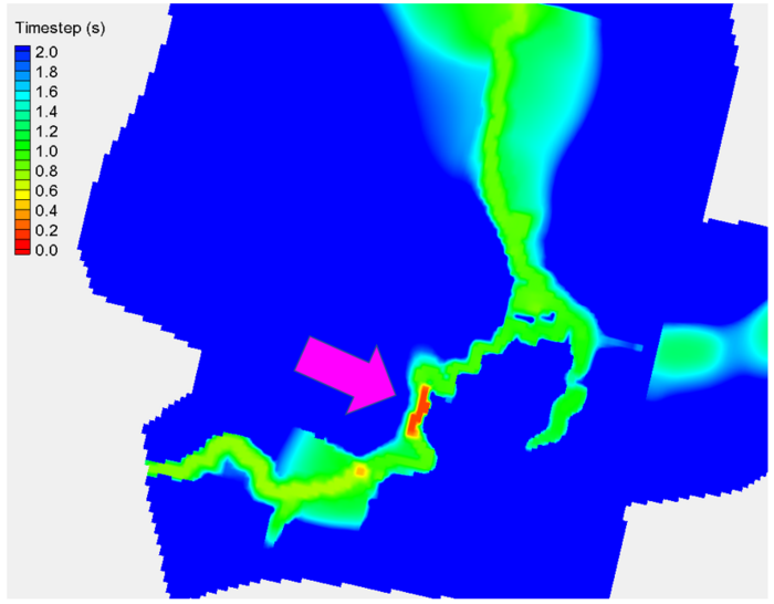
The simulation including the topography error should have run significantly slower (up to 7 times slower). This demonstration highlights how important it is to quality check input datasets to achieve the fastest simulation speed possible using TUFLOW HPC. The new "Minimum dt" map output we added prior to running M03_5m_003.tcf is useful identifying the location that is responsible for the minimum HPC timestep. During real world projects we recommend users review this output and check your model features at the location of minimum timestep to confirm whether the inputs are correct (and should remain) or are an unintended mistake that is inadvertently affecting the simulation speed.
- Open the model results in your preferred viewing package.
- Identify the location of minimum timestep. You should find this corresponds with the data error we introduced for this concept demonstration.
- Open the .tcf file M03_5m_002.tcf and save a copy of the file as M03_5m_004.tcf.
- Add "dt" to the TCF "Map Output Data Types ==" command.
Map Output Data Types == h V q d MB1 MB2 dt
MapInfo Users
- Import the 2d_iwl_empty.mif file from the "mi\empty" folder and save as mi\2d_iwl_M03_004.tab.
- Draw a polygon around the pond in the center of the active model area. Set the "IWL" attribute to 75m. Save and export the file as a MIF/MID file.
- Add the following command to the M03_5m_004.tcf file:
- Read GIS IWL == ..\model\gis\2d_iwl_M03_004.mif ! Read a GIS layer to set initial water level inside polygons
- Open the 2d_iwl_empty_R.shp file from the "gis\empty" folder and save as gis\2d_iwl_M03_004_R.shp.
- Draw a polygon around the pond in the center of the active model area. Set the "IWL" attribute to 75m. Save the file (see the figure above)
- Add the following command to the M03_5m_004.tcf file:
- Read GIS IWL == ..\model\gis\2d_iwl_M03_004_R.shp ! Read a GIS layer to set initial water level inside polygons
- Run the model.
- View the model results in your preferred viewing package. It should be obvious from the results that an incorrect initial water level condition has been applied!
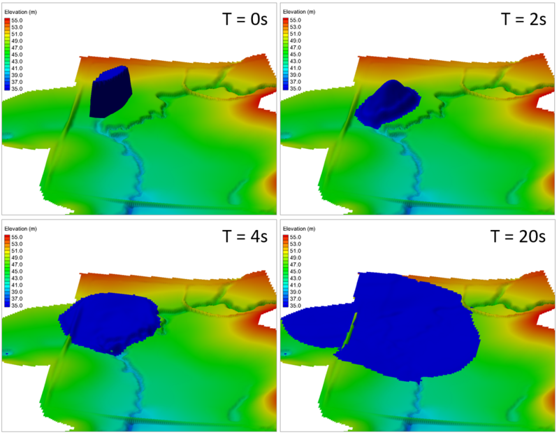
- You can reduce the Map Output Interval in the TCF to a smaller value if you wish to inspect this at a higher refresh rate.
- Open the HPC simulation log files (M03_5m_004.hpc.tlf). Review the model timesteps at the beginning of the simulation. Numerous repeat timesteps should be reported. This highlights instances where TUFLOW HPC had to reduce its step size to remain stable. This is symptomatic of challenging hydraulic conditions and is worth investigation.
- Similar information is also written to the TUFLOW simulation log file. Open M03_5m_004.tlf Review the simulation summary comments at the end of the file.
- Similar to the topography example, the location within the model that is causing the timestep reduction can be identified by viewing the "dt" Map Output results. Open the simulation results in your preferred viewing software. It can be seen that the location of minimum timestep aligns with the feature we used to define the initial water level.
- After completing the TUFLOW HPC simulations, try running the model using TUFLOW Classic instead of TUFLOW HPC. Do this by removing the following commands from the TCF:
- Solution Scheme == HPC
- Hardware == GPU
- Solution Scheme == HPC
- Review simulation results thoroughly; and
- Review the model timestep information as a method to identify possible locations containing data input errors.
Introduction
In this module we add some breaklines to the model to ensure that the 5m cell size model correctly represents the key hydraulic controls. We will add break-lines to represent the following features:
The only new GIS layer that is introduced is the 2d_zshape (2d Z Shape), it is recommended that the user reads section 4.4.9 of the 2010 TUFLOW manual. The 2d_zsh layer is commonly used, and will be also used in later modules.
Note: As per module 2, instructions are given for the following four GIS platforms:
GIS Inputs
For this module you have been provided road crest and creek centreline (thalweg) survey in a text file format (.xyz). This will involve importing the data into a GIS package and then manipulating it into a format suitable for input into TUFLOW. To import the data and manipulate into a TUFLOW format, please select your GIS package from the list below.
Modify Simulation Control Files
With the new GIS layers created it is time to update the control files. The two files we need to change are the geometry control file (.tgc) and the TUFLOW control file (.tcf), the changes for each are described below.
TUFLOW Geometry Control File (TGC)
TUFLOW Control File (TCF)
Run the Simulation
Using your preferred method for starting TUFLOW, run the recently created M03_5m_001.tcf. Please refer to Module 1 for a detailed description of the various methods for running a TUFLOW simulation.
If the model fails to start correctly please refer to the troubleshooting section at the end of this page.
Review Check Files
While the model is running, now is a good time to open the check files to review the changes to the topography caused by the breaklines. As the modifications are to the 2D topography, the check files are written to the TUFLOW\check\2d\ folder.


The check files should show the changes shown above, if they do not please see the troubleshooting section at the bottom of this page.
Review the Results
The 1D and 2D results can be reviewed using the methods outlined in Module 1 and Module 2.
Some suggestions for things to check are:
Conclusion
Point data from survey was provided in text files as x,y,z format data. GIS software was used to import the data and manipulate into a 2d Z Shape format (2d_zsh), the model was simulate with breaklines to represent the creek centre line and road crests.
Check files were used to confirm the changes to the elevation points (Zpts). "Thin", "thick" and "gully" breaklines were described.
The 2D Z Shape can also be used for more complex modifications, using polygons and TIN lines, these will be introduced in later modules.
In Tutorial Module 4 the setup of 1D open channel will be introduced.
Troubleshooting
This section contains links to some possible issue that may occur when progressing through the second tutorial module. If you experience an issue that is not detailed please detail the issue on the discussion page.
If you are unsure of why the model has failed to start, check the TUFLOW Log File (this is in the TUFLOW\runs\log\ folder and has the name M02_5m_001.tlf. This can be opened in a text editor, the error is generally at the end of the file, however you can search for "Error" if you can not see the error.
Advanced - HPC Solver (Optional)
In this optional section we will run the model using the TUFLOW HPC (Heavily Parallelised Compute) solver. TUFLOW HPC can run between 10 and 100 times faster than TUFLOW Classic using NVidia Graphics Processing Units (GPU)(depending on the model configuration and hardware performance).
TUFLOW HPC exhibits unconditional stability. As such, It will automatically select a timestep to maintain simulation stability. This tutorial discusses this feature.
Simulation Using HPC Instead of Classic
Perform the following steps to use TUFLOW's HPC solver instead of TUFLOW Classic:
TIP: If you forget any of the steps, the complete input files are provided as part of the download package (zip file).
TUFLOW HPC Adaptive Timestep Theory
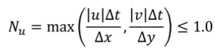
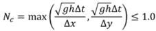
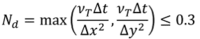
The HPC solver uses adaptive timestepping to progress through the simulation. The timestep is adjusted so that it complies with the mathematical stability criteria of TUFLOW HPC's finite volume explicit solution. The three stability criteria (Control Numbers) are:
where: u is the X-velocity, v the Y-velocity, Δt is the timestep, Δx and Δy are the cell dimensions, g is acceleration, h is water depth and νT is Turbulent Eddy Viscosity. These Control Numbers are kept below 1.0, 1.0 and 0.3, respectively, to stabilise the HPC solver.
The console window below highlights the control numbers and resulting simulation timestep value as for the above simulation. These values will vary during the computation depending on the hydraulic conditions.

Model Timestep Review (Topography Error Example)
In this example We will add a new dataset to demonstrate how topographic data can change the model timestep and simulation speed. The dataset we will use intentionally includes an input error with elevation values set to -99, approximately 140m below the actual ground elevation. Including this dataset in the model will cause TUFLOW HPC to run at a smaller timestep to remain stable.

Complete the following steps:

Model Timestep Review (Boundary Condition Example)
TUFLOW HPC remains stable by using adaptive timestepping (in comparison, Classic uses a fixed timestep). In TUFLOW HPC, if the first timestep estimate violates the celerity, courant or diffusion control numbers or a potential instability is detected, the solution reverts to the previous timestep and repeats the calculation using a smaller step size. This feature makes HPC exceptionally stable and well suited to dam break simulations. Whilst unconditional stability is an attractive feature it also introduces a potential issue. There is risk that accidental input mistakes that would otherwise cause TUFLOW Classic to crash (and bring attention to the input mistake) will remain stable using TUFLOW HPC. With this in mind, careful review of model inputs and results is important using TUFLOW HPC.
The following example demonstrates the exceptional stability of TUFLOW HPC, and the potential risk this poses:


Conclusion
This example highlights the exceptional stability of the TUFLOW HPC solution scheme. This makes it particularly useful for the assessment of challenging dynamic hydraulic conditions, such as dam break scenarios. It can also however pose a potential risk to uneducated users who are more familiar with TUFLOW Classic modelling and expect the software to crash when input datasets containing errors are used. With this in mind, when undertaking TUFLOW HPC model: