Tutorial Module08 Archive
- Apply rainfall over the study area;
- Apply depth-varying roughness for selected landuses; and
- Apply initial and continuing rainfall losses
- Start by opening the materials.csv file found in the TUFLOW\model folder.
- We will be applying depth-varying roughness to three of the landuses within our study area. Amend the second column for Material IDs 1 (pasture), 3 (buildings) and 11 (maintained grass) as shown in the figure below.
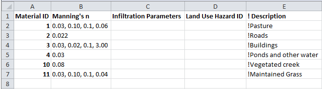
Four numbers (y1, n1, y2, n2) are added to each row separated by commas and are applied as follows; below depth y1 (m or ft) a Manning’s n value of n1 is applied; above y2, n2 is applied, and between y1 and y2, the Manning’s n value is interpolated between n1 and n2. The default interpolation method uses a curved fit so that the n values transition gradually.
For example, for Material ID 1, for depths of water below 0.03m a Manning's n value of 0.10 is applied. For depths of water greater than 0.1m, a Manning's n value of 0.06 is applied. Between 0.03 to 0.1m, a Manning's n value is interpolated between 0.1 and 0.06. For all other Material IDs, the Manning’s n value specified in the second column will be applied at all depths, i.e. a value of 0.022 for Material ID 2.
- Next we will amend the Materials.csv file further to include initial and continuing losses. Amend the third column as shown in the figure below:
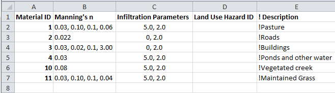
The first number specified in the third column is an initial rainfall loss (in mm or inches). The second number is a continuing rainfall loss (in mm/hr or inches/hr).
Note that these rainfall losses applied through a materials definition file use a rainfall excess approach. As such the rainfall losses are subtracted from the input hyetograph prior to being applied to the model as a boundary on 2D cells. This is different to losses specified using a TUFLOW soils file (.tsoilf). Rainfall losses applied using a TUFLOW soils file (.tsoilf) extracts water from model via infiltration from wet 2D cells.
- Save the file as materials_depth_varying.csv. It is now ready to be used in the model.
- We have created a new 2d_rf layer to read in direct rainfall over our proposed development.
- Begin by opening M07_5m_001.tbc in your text editor. Save the file as M08_5m_001.tbc.
- Within the first If Scenario, change 'DEV' to 'DEV|EXG'. In the following Else If Scenario statement, delete 'EXG' from the line. The vertical bar "|" allows you to include additional scenarios into the current IF statement without the need to create a new one.
- Comment out the Read GIS SA PITS command within the If Scenario logic block and the Read GIS SA command by placing an exclamation mark "!" at the beginning of the lines. The commands will now be treated as comments and ignored by TUFLOW.
- Within the If Scenario logic block and after the commented out line !Read GIS SA PITS == mi\2d_sa_M07_001.MIF add the following:
MapInfo Users
Read GIS RF == mi\2d_rf_M08_001.MIF
QGIS or ArcGIS Users
Read GIS RF == gis\2d_rf_M08_001_R.SHP
Tip - indenting commands within your If Scenario statements makes your model more readable - Save the file. The tbc file is now ready to be used.
- Open M07_5m_~s1~_001.tcf and save as M08_5m_~s1~_001.tcf.
- Update the following commands:
BC Control File == ..\model\ M08_5m_001.tbc
BC Database == ..\bc_dbase\bc_dbase_M08_001.csv
Read Materials File == ..\model\Materials_depth_varying.csv
- We will also specify a new output folder for the results of this module:
Output Folder == ..\results\M08\2d
- Lastly, we will write additional map outputs so we can view how Manning’s n, cumulative rainfall (RFC) and rainfall rate (RFR) values change over time. Update the following command:
Map Output Data Types == h V q d n RFC RFR
- Save the file. The tcf file is now ready to be used.
- Open the TLF in a text editor. The file is located in the TUFLOW\runs\log folder.
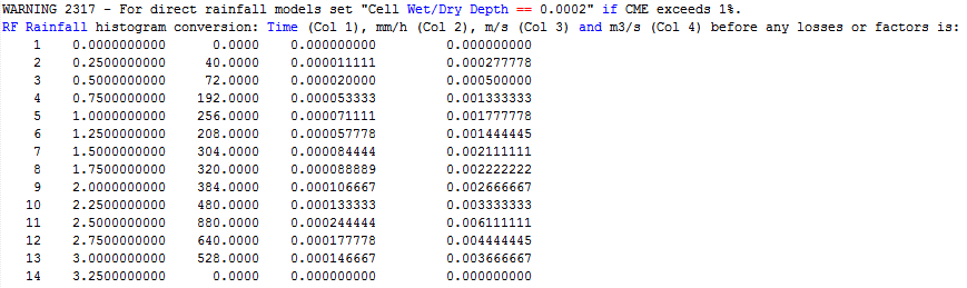
- Review the hyetograph information. The tlf file shows the hyetograph read into the model and its conversion to a hydrograph.
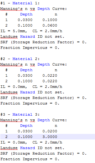
- Review the depth-varying roughness and rainfall loss information. The figure below shows a sample of the information provided in the TLF.
- M08_5m_001_MB1D.csv: Mass balance reporting for all 1D domains
- M08_5m_001_MB2D.csv: Mass balance reporting for all 2D domains
- M08_5m_001_MB.csv: Mass balance reporting for the overall model (1D and 2D domains)
- Adjustment of the Cell Wet/Dry depth parameter; and
- Simulation using the double precision version of TUFLOW.
- Open the file M08_5m_~s1~_001.tcf found within the TUFLOW\Runs folder and save as M08_5m_~s1~_002.tcf. Add the following commands anywhere within the .tcf:
Cell Wet/Dry Depth == 0.0002
So far we have been using the Single Precision version of TUFLOW for our simulations. This can be confirmed in the screenshot above of the _ TUFLOW Simulations.log file.
The Double Precision version of TUFLOW is recommended for all direct rainfall models.
The double precision version uses a great number of significant figures in it's calculations than the single precision version and is required for direct rainfall models due to the shallow depth of flow. At these shallow depths, more significant figures are needed to prevent mathematic rounding from producing mass error. For more information on single vs double precision, refer to this Wiki page.
- Add the following command anywhere within M08_5m_~s1~_002.tcf.
Model Precision == Double
Inclusion of this Model Precision command will ensure the model is always simulated using the correct version of TUFLOW. If the model is simulated with a version other than that intended, the simulation will be stopped and an error output.
- The final changes we need to make are to the batch file. Update the file with the changes highlighted in red. These will call the double precision version of TUFLOW and also run the base case (EXG) and developed case (DEV) scenario models in sequence one after another.
set TUFLOWEXE_iSP=C:\TUFLOW\Releases\2017-09-AC\w64\TUFLOW_iSP_w64.exe set TUFLOWEXE_iDP=C:\TUFLOW\Releases\2017-09-AC\w64\TUFLOW_iDP_w64.exe
set RUN_iSP=start "TUFLOW" /wait "%TUFLOWEXE_iSP%" -b set RUN_iDP=start "TUFLOW" /wait "%TUFLOWEXE_iDP%" -b
%RUN_iDP% -s1 EXG M08_5m_~s1~_002.tcf %RUN_iDP% -s1 DEV M08_5m_~s1~_002.tcf - Save the .tcf and batch files and re-run the model.
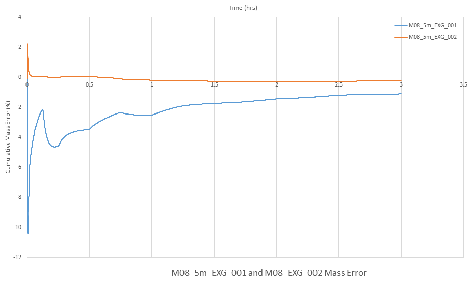
- Once the model has finished simulating, open the M08_5m_002_MB.csv file and plot the Cum ME (%) column. The results should show a reduction in CME to within the recommended range of +/-1%.
- Save the TUFLOW runfile M08_5m_~s1~_002.tcf as M08_5m_~s1~_003.tcf.
- Add the following command to the tcf file:
- Solution Scheme == HPC ! Use the HPC solver to run the model
- Solution Scheme == HPC ! Use the HPC solver to run the model
- If you have a CUDA enabled NVIDIA GPU device, you can also add the following command to run the HPC solver using GPU hardware:
- Hardware == GPU ! Run HPC solver on GPU
- Hardware == GPU ! Run HPC solver on GPU
- Delete or comment out the command Model Precision == Double.
TUFLOW HPC uses a different solution scheme to TUFLOW Classic. It has been tailor made for direct rainfall applications and does not required double precision. Single precision is recommended when using TUFLOW HPC.
- ! Model Precision == Double
- ! Model Precision == Double
- Save the tcf file.
- Update the batch file with the changes highlighted below in red. The batch file will run four models in sequence, base case (EXG) and developed case (DEV) scenario simulations using TUFLOW Classic and TUFLOW HPC. It will call the double precision version of TUFLOW for TUFLOW Classic. It will call the single precision version of TUFLOW for TUFLOW HPC simulations.
set TUFLOWEXE_iSP=C:\TUFLOW\Releases\2017-09-AC\w64\TUFLOW_iSP_w64.exe
set TUFLOWEXE_iDP=C:\TUFLOW\Releases\2017-09-AC\w64\TUFLOW_iDP_w64.exe

set RUN_iSP=start "TUFLOW" /wait "%TUFLOWEXE_iSP%" -b
set RUN_iDP=start "TUFLOW" /wait "%TUFLOWEXE_iDP%" -b

%RUN_iDP%    -s1    EXG    M08_5m_~s1~_002.tcf
%RUN_iDP%    -s1    DEV    M08_5m_~s1~_002.tcf

%RUN_iSP%    -s1    EXG    M08_5m_~s1~_003.tcf
%RUN_iSP%    -s1    DEV    M08_5m_~s1~_003.tcf
- Run the TUFLOW Classic and HPC simulations.
- Review the results.
- Also, to learn how to optimise a HPC simulation to achieve the fastest simulation speed please complete Tutorial Module 2 and Tutorial Module 3
- Check if your GPU card is an NVIDIA GPU card. Currently, TUFLOW does not run on AMD type GPU.
- Check if your NVIDIA GPU card is CUDA enabled and whether the latest drivers are installed. Please see GPU Setup.
Introduction
In this module we will further develop the model from Module 07. We will be developing a direct rainfall model where a rainfall hyetograph is applied to all active cells within the model boundary. This hyetograph (rainfall versus time) will replace the hydrograph (flow versus time) inflow boundary used in previous modules.
In this tutorial we will be changing the main river flow to a constant base flow and focusing on the direct rainfall.
The steps we will be completing in this tutorial are:
GIS and Model Inputs
The steps necessary to modify each of the GIS inputs are demonstrated in MapInfo, ArcGIS and QGIS. At each stage please select your GIS package to view relevant instructions. For this tutorial a hyetograph and polygon representing the rainfall area has been provided.
Direct Rainfall
This part of the tutorial will demonstrate how to apply direct rainfall to a model. We will also create a new boundary conditions database to reference the hyetograph. Follow the instructions below for your preferred GIS package.
Depth Varying Roughness and Rainfall Losses
This part of the module will demonstrate how depth-varying roughness and rainfall losses can be applied to landuses specified within the model.


Modify Simulation Control Files
Now that we have made all of the necessary changes to the GIS layers, we need to update our control files. We will incorporate the direct rainfall changes into the base ('EXG') and developed ('DEV') cases introduced in Module 7.
TBC
There has been one change to the model that impacts the boundary conditions of the model:
Tip: Refer to the M08_5m_001.tbc file within the Complete_Model download dataset if you require an example of the above update.
TCF
We will need to create a new tcf file that references the new tbc, bc_dbase, and materials.csv files.
Run Simulation
Using your preferred method for starting TUFLOW, run the newly created M08_5m_~s1~_001.tcf. Please refer to Module 1 for a detailed description of the various methods for running a TUFLOW simulation.
In this tutorial we are using a batch file to run simulations. The command line in our batch file will be similar to that used in Module 7:
set TUFLOWEXE_iSP=C:\TUFLOW\Releases\2017-09-AC\w64\TUFLOW_iSP_w64.exe set RUN_iSP=start "TUFLOW" /wait "%TUFLOWEXE_iSP%" -bb |
If the model fails to start correctly please refer to the troubleshooting section at the end of this page.
Tip: An example batch file called _ run all simulations.bat is included in the runs folder of the Complete_Model download dataset.
Review Model Updates
Once the model has compiled and the simulation started, we can review the TUFLOW Log File (TLF) to ensure the changes we have made have been correctly applied.


Review Model Health
Once the TUFLOW Classic simulation has finished, it is good practice to view the Cumulative Mass Error (CME) of the model as a measure of its health. The CME may be viewed in a number of different ways. The _ TUFLOW Simulations.log file written to the TUFLOW\runs folder, provides a summary of CME along with other information such as the name of the computer used to run the model and the TUFLOW build used. The figure below shows the output from the log file for our model simulation. The value highlighted is the peak CME throughout the whole simulation. The value of -10.42% is well outside the recommended range of +/-1% and tells us the CME needs to be looked into in more detail.
![]()
Three csv files providing further information on CME have also been written to the TUFLOW\results\1D and TUFLOW\results\M08\2D folders. These are:
Opening the M07_5m_001_MB.csv file and plotting the Cum ME (%) column produces the figure below. The high CME values are seen to occur in the first half hour of our simulation

The high CME values in our model are due to some fundamental changes to the run parameters that need to be incorporated for all direct rainfall models. These are:
You may have spotted in the figure of the tlf file above that a message was outputted:
“WARNING 2317 - For direct rainfall models set "Cell Wet/Dry Depth == 0.0002" if CME exceeds 1%.”
As with all checks, warnings and errors, further information can be found on the TUFLOW Message Database. More information on this message specifically can be found here. The Cell Wet/Dry Depth command specifies the depth at the cell in which TUFLOW transitions from wet to dry and vice versa. The depth should be selected according to the magnitude of flooding depths. As direct rainfall models typically have a high proportion of shallow sheet flow, a wet/dry depth of less than 1mm (eg. 0.0002m) may be required.

View the Results
Open the 2D results in your preferred results viewer or import to your GIS package. For more information on how to do this, refer to Module 1.
This module has applied the rainfall boundary to every active 2D cell. To aid visualisation of the results, an appropriate cut-off depth is typically used to only display the results above the specified depth. The depth chosen differentiates between shallow, sheet flow and depths classed as 'flooded'. The cut-off can be specified directly in the tcf or through post-processing of the results. 0.1m is commonly used as the cutoff depth value. The TCF command for TUFLOW to do this is:
Map Cutoff Depth == 0.10
The below image shows the maximum predicted flood depth for the base case (EXG) scenario, with a cut-off depth of 0.1m applied.

To post process the gridded results with a cut-off depth, the asc_to_asc utility may be used.
Visualising the velocity vectors in direct rainfall models provides a means to investigate flow paths and their behaviour. Note in the below image that a cut-off depth has been applied to the depth grid, but not the velocity vectors, thus the velocity and direction of shallow sheet flow can still be seen.

This model has allowed for the Manning's n roughness values for select landuses to vary with flood depth. This variation over time may be visualised by viewing the 'n' map output type. This additional dataset is located with the simulation results (n.dat or within the xmdf file) and can be visualised using the same methods as for all other map output types. The below image is a snapshot of the manning's 'n' value at 1.6hrs into the simulation.

Cumulative rainfall (RFC) and rainfall rate (RFR) Map Output Data was also added to this model. These outputs will track the rainfall in mm/hr (RFR) and the total rainfall depth applied to the model over time (RFC). View these results in your preferred results viewing software.

HPC Solver (Optional)
In this optional section we will run the model using TUFLOW HPC (Heavily Parallelised Compute). TUFLOW HPC can run between 10 and 100 times faster than TUFLOW Classic using NVidia Graphics Processing Units (GPU)(depending on the model configuration and hardware performance). The speed of HPC makes it exceptionally well suited to high resolution direct rainfall urban applications. Large models with over 1,000,000 2D cells that take days to run using TUFLOW Classic can take hours to complete using TUFLOW HPC with high performance GPU hardware! The presentation "Rapid and Accurate Stormwater Drainage Assessments Using GPU Technology" highlights some performance test results comparing TUFLOW Classic against TUFLOW HPC for high resolution direct rainfall urban 1D/2D applications. A pdf copy of the presentation is available from the TUFLOW Library
Note: If you have not previously used TUFLOW HPC, we recommend completing Tutorial Module 1, 2 and 3 before attempting this tutorial. The preceding tutorials include important lessons specific to using HPC, particularly its adaptive timestep / unconditional stability and GPU Hardware.
In order to use the HPC solver, we will need to perform the following steps:
TIP: To switch on the HPC solver via scenario control commands, please see the HPC Model Setup section of Module 5 (recommended).
Conclusion
In this module, we have applied direct rainfall over the model. We have specified depth-varying roughness and rainfall losses to selected landuses. This module highlights the need to lower the Cell Wet/Dry Depth and use the Double Precision version of TUFLOW for the TUFLOW Classic direct rainfall models. TUFLOW HPC should use the Single Precision version of TUFLOW for direct rainfall applications.
Troubleshooting
If the TUFLOW simulation fails to start TUFLOW will output the error in a number of locations. Firstly, check the Console Window or the TUFLOW Log File (.tlf) (located in the TUFLOW\runs\log\ folder). This file can be opened in a text editor and the error is generally located at the end of the file. You can however search for "Error" if you cannot see the error. In most cases there is also a spatial location for the error message (if the error reported in the log file is prefixed by XY:). To check the location of the geographic errors, open the _messages.mif or _messages_P.shp file in your GIS package.
This section contains links to some possible problems that may occur when progressing through the fourth tutorial module. If you experience an issue that is not detailed, please email support@tuflow.com or add and describe the problem on the discussion page.
If you receive the following error when trying to run the TUFLOW HPC model using GPU hardware:
TUFLOW GPU: Interrogating CUDA enabled GPUs …
TUFLOW GPU: Error: Non-CUDA Success Code returned
or
ERROR 2785 - No GPU devices found, enabled or compatible.
Please try the following steps: