HPC Model Review: Difference between revisions
| (30 intermediate revisions by 4 users not shown) | |||
| Line 1: | Line 1: | ||
= Introduction = |
= Introduction = |
||
HPC is an unconditionally stable 2D solution scheme that is mass conservative. This can result in HPC “hiding” poor data or model setup. Modellers must take measures to ensure the quality of their HPC models for commercial uses, by taking all reasonable steps to correct or at the very least understand areas of poor representation in their models.<br> |
TUFLOW HPC is an unconditionally stable 2D solution scheme that is mass conservative. This can result in HPC “hiding” poor data or model setup. Modellers must take measures to ensure the quality of their HPC models for commercial uses, by taking all reasonable steps to correct or at the very least understand areas of poor representation in their models.<br> |
||
= TUFLOW Log |
= TUFLOW Log File (*.tlf) = |
||
The first step of reviewing a HPC model is no different to reviewing a TUFLOW Classic model. Start by opening the TUFLOW log file (*.tlf) and confirm at the bottom of the file, that the model run finished successfully by observing "Simulation FINISHED" and that the final mass error reported is acceptable as shown below:<br> |
The first step of reviewing a HPC model is no different to reviewing a TUFLOW Classic model. Start by opening the TUFLOW log file (*.tlf) and confirm at the bottom of the file, that the model run finished successfully by observing "Simulation FINISHED" and that the final mass error reported is acceptable as shown below:<br> |
||
[[ |
[[File:Simulation Summary 02.PNG]]<br> |
||
Though HPC is mass |
Though HPC is volume conservative and shouldn't produce any mass error it is still important to review the Mass Error, as it can still occur when coupling HPC with 1D elements in either the 1D/2D linking, or in the 1D itself.<br> |
||
A 'healthy' model will usually report up to |
A 'healthy' model will usually report up to 1% mass error. Higher mass error is an indication the solution is not converging, usually in isolated locations. In nearly all cases it is because of poor data (e.g. cliff edge between data sets) or model schematisation (e.g. large pit connected to one tiny 2D cell or boundary poorly digitised so it is not roughly perpendicular to the flow). The total model mass error can also be observed in the TUFLOW Summary File (*.tsf) output as oppose to the tlf file. <br> |
||
| ⚫ | |||
= HPC TUFLOW Log File (*hpc.tlf) = |
|||
The .hpc.tlf log file records the model timestep, control numbers and volume of water in model at each timestep. It also shows repeated timesteps if the <u>[[HPC_Adaptive_Timestepping | control number limits]]</u> were exceeded or there is a significant change in control numbers (more than 20%). It is inevitable to have repeated timesteps, if a model has a sudden change in rainfall input from one timestep to the next, or has a warmup period with small flow rate before a large inflow. However, if there is a high occurrence of repeating timesteps when the boundary inflows are smooth, this could be an indicator of model instability. The total number of repeated timesteps is also recorded in Simulation Summary of the .tlf file.<br> |
|||
'''Note:''' TUFLOW HPC allows the <u>[[HPC_Adaptive_Timestepping | control numbers]]</u> to be breached by 20%. The timestep will not be repeated with Nc, Nu smaller than 1.2 and Nd smaller than 0.36. <br> |
|||
<br> |
|||
[[File: HPC_repeating_timestep.png]] |
|||
| ⚫ | |||
The last column of the *hpc.tlf file records the timesteping efficiency output. A value of 100% indicates that the HPC timesteps are perfectly aligned with the minimum stability timestep for complying with the three control numbers representing the Courant, Wave Celerity and Diffusion criteria.<br> |
|||
If virtual pipes are used in the model, the following information will also be reported in the hpc.tlf and console window: |
|||
* qInlet: flow extracted from the 2D domain. |
|||
* qSurcharge: flow surcharging out of inlets, due to the outlet flow being limited. |
|||
* qOutput: flow entering the 2D domain. |
|||
= HPC dt Time Series Output (*.hpc.dt.csv) = |
= HPC dt Time Series Output (*.hpc.dt.csv) = |
||
This csv output provides a timeseries of the model timestep and the value of each control number at each timestep.<br> |
|||
[[File: Hpc_dt_csv.png |450px]] |
|||
<br> |
|||
It is recommended that modellers review the hpc.dt.csv file to check the dt timeseries output. There are two key features that modellers should look for in the hpc.dt.csv output, one is erratic bouncing of the dt values and the second is extremely low dt values. Anything less than 1/10 of a healthy TUFLOW Classic timestep could be consider low, but could vary depending on the study, for example a dam break assessment with high velocities and depths may require a much lower timestep. This becomes easier to observe by graphing the dt timeseries as shown below.<br> |
It is recommended that modellers review the hpc.dt.csv file to check the dt timeseries output. There are two key features that modellers should look for in the hpc.dt.csv output, one is erratic bouncing of the dt values and the second is extremely low dt values. Anything less than 1/10 of a healthy TUFLOW Classic timestep could be consider low, but could vary depending on the study, for example a dam break assessment with high velocities and depths may require a much lower timestep. This becomes easier to observe by graphing the dt timeseries as shown below.<br> |
||
| Line 19: | Line 38: | ||
If bouncing or an unusually low timestep is observed in the HPC dt time series it is important to also review the value associated with for each control number (Nu, Nc and Nd). This will allow the modeller to determine which hydraulic condition is limiting the timestep most. In the example below, the Wave Celerity condition is reducing the timestep as shown by the highlighted Nc value of 0.999.<br> |
If bouncing or an unusually low timestep is observed in the HPC dt time series it is important to also review the value associated with for each control number (Nu, Nc and Nd). This will allow the modeller to determine which hydraulic condition is limiting the timestep most. In the example below, the Wave Celerity condition is reducing the timestep as shown by the highlighted Nc value of 0.999.<br> |
||
[[FILE: Hpc_log_file.png |
[[FILE: Hpc_log_file.png]] |
||
This becomes valuable when trying to determine what is causing the low timestep and how to resolve it. For example:<br> |
This becomes valuable when trying to determine what is causing the low timestep and how to resolve it. For example:<br> |
||
| ⚫ | |||
| ⚫ | |||
*An Nu value of 1.0 or greater may indicate that the velocity is unusually high. |
*An Nu value of 1.0 or greater may indicate that the velocity is unusually high. |
||
| ⚫ | |||
| ⚫ | |||
Because each relates to a hydraulic condition, they provide insight into what might be causing an issue in the model.<br> |
Because each relates to a hydraulic condition, they provide insight into what might be causing an issue in the model.<br> |
||
= dt Map Output = |
= dt Map Output = |
||
The dt map output is a grid map output that displays the calculated minimum timestep at each grid cell, and does not necessarily align with the timestep adopted in the model (the timestep in the model could be less if the previous timesteps were smaller). This helps identify which cells in the model are controlling the model timestep.<br> |
|||
<font color="blue"><tt>Map Output Data Types </tt></font><font color="red"><tt>==</tt></font><tt> dt </tt> writes the minimum dt (timestep) calculated for each cell in the model to the specified Map Output Format (XMDF, DAT, ASC, FLT etc.). Reviewing this output helps modellers identify which cells in the model have the lowest timestep and thereby control the model timestep. These locations are likely to have the greatest depth, velocity or turbulence in the model, forcing TUFLOW to lower the timestep to satisfy the conditions of the controlling numbers mentioned in the <u>[[HPC_Adaptive_Timestepping | HPC Adaptive Timestepping]]</u> page. If the timestep is extremely low the HPC model might be “hiding” poor data or model setup in this location.<br> |
<font color="blue"><tt>Map Output Data Types </tt></font><font color="red"><tt>==</tt></font><tt> dt </tt> writes the minimum dt (timestep) calculated for each cell in the model to the specified Map Output Format (XMDF, DAT, ASC, FLT etc.). Reviewing this output helps modellers identify which cells in the model have the lowest timestep and thereby control the model timestep. These locations are likely to have the greatest depth, velocity or turbulence in the model, forcing TUFLOW to lower the timestep to satisfy the conditions of the controlling numbers mentioned in the <u>[[HPC_Adaptive_Timestepping | HPC Adaptive Timestepping]]</u> page. If the timestep is extremely low the HPC model might be “hiding” poor data or model setup in this location. The simulation timestep will always be limited by the minimum occurring timestep anywhere in the model, hence it is important to ensure timestepping isn’t being unnecessarily restricted due to poor model configuration in one spot, even only in one cell. <br> |
||
<br> |
|||
| ⚫ | |||
<br> |
<br> |
||
| ⚫ | |||
The cause of the low timestep may become clearer when observing it geographically in the dt Map Output, as the low timestep may occur close to specific hydraulic features. This is seen in the example above, where an unusually low dt value is observed upstream, where the road intersects a local channel. It is helpful to review this in conjunction with the hpc.dt.csv to know which of the controlling numbers is causing the timestep to be lowered.<br> |
The cause of the low timestep may become clearer when observing it geographically in the dt Map Output, as the low timestep may occur close to specific hydraulic features. This is seen in the example above, where an unusually low dt value is observed upstream, where the road intersects a local channel. It is helpful to review this in conjunction with the hpc.dt.csv to know which of the controlling numbers is causing the timestep to be lowered.<br> |
||
<br> |
|||
'''Note:''' Be aware that some mapping programs will automatically display a raster only within a given percentage bounds, and may need to be set to show the full range of values.<br> |
|||
<br> |
|||
[[FILE: QGIS_raster_display_accuracy.png]] <br> |
|||
= Velocity and Velocity Vector Output = |
= Velocity and Velocity Vector Output = |
||
| Line 48: | Line 73: | ||
= Control Number Factor Sensitivity Testing = |
= Control Number Factor Sensitivity Testing = |
||
Sensitivity run can be done by reducing timestepping interval using Control Number Factor == 0.8. This reduces the timestep (as dictated by the three control numbers) by the factor 0.8, making the simulation to take roughly 20% longer. If comparing the two results shows negligible differences it is a strong indicator the default control number limits may be considered satisfactory. If there are unacceptable measurable differences, the location of these impacts may also help to spatially identify where the solution may have been struggling at the default control numbers. These areas can then be inspected for input topography or boundary conditions errors. Models shouldn’t need to have the CNF lowered any more than this, as if they do, it would indicate there is more likely an underlying model configuration issue that needs attention. |
Sensitivity run can be done by reducing timestepping interval using Control Number Factor == 0.8. This reduces the timestep (as dictated by the three control numbers) by the factor 0.8, making the simulation to take roughly 20% longer. If comparing the two results shows negligible differences it is a strong indicator the default control number limits may be considered satisfactory. If there are unacceptable measurable differences, the location of these impacts may also help to spatially identify where the solution may have been struggling at the default control numbers. These areas can then be inspected for input topography or boundary conditions errors. Models shouldn’t need to have the CNF lowered any more than this, as if they do, it would indicate there is more likely an underlying model configuration issue that needs attention. |
||
<br> |
|||
<br> |
|||
{{Tips Navigation |
|||
|uplink=[[ HPC_Modelling_Guidance | Back to HPC Modelling Guidance]] |
|||
}} |
|||
Latest revision as of 22:17, 12 July 2024
Introduction
TUFLOW HPC is an unconditionally stable 2D solution scheme that is mass conservative. This can result in HPC “hiding” poor data or model setup. Modellers must take measures to ensure the quality of their HPC models for commercial uses, by taking all reasonable steps to correct or at the very least understand areas of poor representation in their models.
TUFLOW Log File (*.tlf)
The first step of reviewing a HPC model is no different to reviewing a TUFLOW Classic model. Start by opening the TUFLOW log file (*.tlf) and confirm at the bottom of the file, that the model run finished successfully by observing "Simulation FINISHED" and that the final mass error reported is acceptable as shown below:
Though HPC is volume conservative and shouldn't produce any mass error it is still important to review the Mass Error, as it can still occur when coupling HPC with 1D elements in either the 1D/2D linking, or in the 1D itself.
A 'healthy' model will usually report up to 1% mass error. Higher mass error is an indication the solution is not converging, usually in isolated locations. In nearly all cases it is because of poor data (e.g. cliff edge between data sets) or model schematisation (e.g. large pit connected to one tiny 2D cell or boundary poorly digitised so it is not roughly perpendicular to the flow). The total model mass error can also be observed in the TUFLOW Summary File (*.tsf) output as oppose to the tlf file.
HPC TUFLOW Log File (*hpc.tlf)
The .hpc.tlf log file records the model timestep, control numbers and volume of water in model at each timestep. It also shows repeated timesteps if the control number limits were exceeded or there is a significant change in control numbers (more than 20%). It is inevitable to have repeated timesteps, if a model has a sudden change in rainfall input from one timestep to the next, or has a warmup period with small flow rate before a large inflow. However, if there is a high occurrence of repeating timesteps when the boundary inflows are smooth, this could be an indicator of model instability. The total number of repeated timesteps is also recorded in Simulation Summary of the .tlf file.
Note: TUFLOW HPC allows the control numbers to be breached by 20%. The timestep will not be repeated with Nc, Nu smaller than 1.2 and Nd smaller than 0.36.

The new *hpc.tlf file can be also used to review the dt, controlling number values and the water volume in the model. However, this may be easier to review using the hpc.dt.csv output.
The last column of the *hpc.tlf file records the timesteping efficiency output. A value of 100% indicates that the HPC timesteps are perfectly aligned with the minimum stability timestep for complying with the three control numbers representing the Courant, Wave Celerity and Diffusion criteria.
If virtual pipes are used in the model, the following information will also be reported in the hpc.tlf and console window:
- qInlet: flow extracted from the 2D domain.
- qSurcharge: flow surcharging out of inlets, due to the outlet flow being limited.
- qOutput: flow entering the 2D domain.
HPC dt Time Series Output (*.hpc.dt.csv)
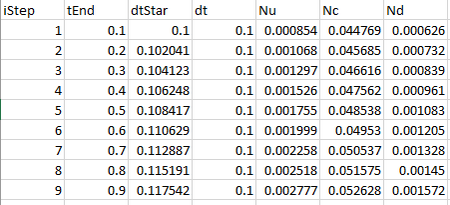
This csv output provides a timeseries of the model timestep and the value of each control number at each timestep.
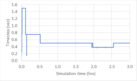
It is recommended that modellers review the hpc.dt.csv file to check the dt timeseries output. There are two key features that modellers should look for in the hpc.dt.csv output, one is erratic bouncing of the dt values and the second is extremely low dt values. Anything less than 1/10 of a healthy TUFLOW Classic timestep could be consider low, but could vary depending on the study, for example a dam break assessment with high velocities and depths may require a much lower timestep. This becomes easier to observe by graphing the dt timeseries as shown below.
Observing either bouncing of the dt, or an extremely low dt value in the timeseries may indicate that modelling issues are being resolved by HPC’s solution scheme. This could lead to results that misrepresent the hydraulic behavior in that area. To determine where in the model these low timesteps are occurring, the dt Map Output can be used.
If bouncing or an unusually low timestep is observed in the HPC dt time series it is important to also review the value associated with for each control number (Nu, Nc and Nd). This will allow the modeller to determine which hydraulic condition is limiting the timestep most. In the example below, the Wave Celerity condition is reducing the timestep as shown by the highlighted Nc value of 0.999.
This becomes valuable when trying to determine what is causing the low timestep and how to resolve it. For example:
- An Nu value of 1.0 or greater may indicate that the velocity is unusually high.
- An Nc value of 1.0 or higher could be caused by an erroneously low cell elevation, resulting in an artificially large water depth.
- An Nd value of 0.3 or higher might suggest that there is poor boundary setup, or insufficient SX cells linked to a 1D structure.
Because each relates to a hydraulic condition, they provide insight into what might be causing an issue in the model.
dt Map Output
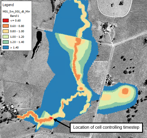
The dt map output is a grid map output that displays the calculated minimum timestep at each grid cell, and does not necessarily align with the timestep adopted in the model (the timestep in the model could be less if the previous timesteps were smaller). This helps identify which cells in the model are controlling the model timestep.
Map Output Data Types == dt writes the minimum dt (timestep) calculated for each cell in the model to the specified Map Output Format (XMDF, DAT, ASC, FLT etc.). Reviewing this output helps modellers identify which cells in the model have the lowest timestep and thereby control the model timestep. These locations are likely to have the greatest depth, velocity or turbulence in the model, forcing TUFLOW to lower the timestep to satisfy the conditions of the controlling numbers mentioned in the HPC Adaptive Timestepping page. If the timestep is extremely low the HPC model might be “hiding” poor data or model setup in this location. The simulation timestep will always be limited by the minimum occurring timestep anywhere in the model, hence it is important to ensure timestepping isn’t being unnecessarily restricted due to poor model configuration in one spot, even only in one cell.

The cause of the low timestep may become clearer when observing it geographically in the dt Map Output, as the low timestep may occur close to specific hydraulic features. This is seen in the example above, where an unusually low dt value is observed upstream, where the road intersects a local channel. It is helpful to review this in conjunction with the hpc.dt.csv to know which of the controlling numbers is causing the timestep to be lowered.
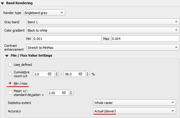
Note: Be aware that some mapping programs will automatically display a raster only within a given percentage bounds, and may need to be set to show the full range of values.

Velocity and Velocity Vector Output
Check for any unusually high velocities in the maximum and temporal output. Review of velocity vectors can also be useful when styled Scaled to Magnitude in a GIS package.
Water Level Output
Look for “bumps” or “monds” in the maximum water level surface. One way to do this is by generating water level contours at, say, 0.1m intervals and panning around looking for any bumps. Alternatively, appropriate shading settings will also work. As the maximum surface values are being tracked every timestep, if there is a numerical bounce, it will be recorded and propagate away from the location creating the bump or mound. Typically Classic, with its fixed timestep, nearly always goes unstable if a bounce occurs and the simulation stops with error. However, HPC with its adaptive timestepping can recover from the bounce and continue simulating. Thus a sudden, change in timestepping (not associated with approaching an output interval) is evidence of a possible bounce. But by far, the best way of reviewing (for any 2D software) is to check there are no bumps or mounds across the maximum water level surface as a result of a bounce, especially for adaptive timestepping solutions due to their ability to recover and not go unstable. Checking the water level surfaces at instants in time is also an option noting that a bounce may have occurred between map output times. If bumps or mounds are evident then try using smaller timestepping by reducing control number factor.
Time Series Output
Review _TS results for unusually high values in 1D engine ESTRY.
PO Output
Time-series PO water level and flow lines across the whole waterway at key locations are always useful. If these are numerically oscillating, it can be an indicator of numerical instabilities.
Control Number Factor Sensitivity Testing
Sensitivity run can be done by reducing timestepping interval using Control Number Factor == 0.8. This reduces the timestep (as dictated by the three control numbers) by the factor 0.8, making the simulation to take roughly 20% longer. If comparing the two results shows negligible differences it is a strong indicator the default control number limits may be considered satisfactory. If there are unacceptable measurable differences, the location of these impacts may also help to spatially identify where the solution may have been struggling at the default control numbers. These areas can then be inspected for input topography or boundary conditions errors. Models shouldn’t need to have the CNF lowered any more than this, as if they do, it would indicate there is more likely an underlying model configuration issue that needs attention.
| Up |
|---|


