TUFLOW Remapping: Difference between revisions
No edit summary |
|||
| (34 intermediate revisions by 4 users not shown) | |||
| Line 1: | Line 1: | ||
<poem lang="fr" style="float:left;"> |
|||
The 2020 release of TUFLOW included new Quadtree mesh and Sub-grid Sampling (SGS) functionality. The SGS feature now supports the |
|||
hydraulic analysis of partially wet cells on the flood fringe. Currently, cells that are partially wet are displayed in model output |
|||
as being fully wet. This page introduces how to use the ASC_to_ASC remap function, and discusses limitations of the method.</poem><br><br> |
|||
[[File: Remap_Advice_LinkedIn.jpg ||450px|right]] |
|||
<br><br><br><br><br><br> |
|||
__TOC__ |
|||
= Introduction = |
= Introduction = |
||
With the release of TUFLOW 2020, the combination of Quadtree mesh and Sub-grid Sampling (SGS) method has offered great flexibility |
With the release of TUFLOW 2020, the combination of Quadtree mesh and Sub-grid Sampling (SGS) method has offered great flexibility for rapidly building flood models of varying resolution and increased topographic detail. Now a wide range of mesh sizes can be applied in a model based on the geographic feature and the area of interest in a project. Especially with the SGS method, cells and faces can be treated as 'partially wet', and the impact of the sub-grid scale geometry may be represented by cells with larger sizes.<br> |
||
The example below shows that a Quadtree model with 10/20m cell size (right) can convey water as smoothly as a 2.5/5/10/20m model along the narrow and meandering gully line.<br> |
|||
[[File:Fig1 H sgs.png|700px]]<br> |
[[File:Fig1 H sgs.png|700px]]<br> |
||
'''Figure 1 Water level simulation results with SGS. Left: 2.5/5/10/20m Quadtree model. Right: 10/20m Quadtree model.'''<br><br> |
'''Figure 1 Water level simulation results with SGS. Left: 2.5/5/10/20m Quadtree model. Right: 10/20m Quadtree model.'''<br><br> |
||
On the other hand, the same model running without SGS |
On the other hand, the same model running without SGS applied creates notably different results in the distance of water travelled and the area of inundation on the floodplain due to the poor topographic representation (one elevation per cell centre and cell face).<br> |
||
[[File:Fig2 H nonsgs.png|700px]]<br> |
[[File:Fig2 H nonsgs.png|700px]]<br> |
||
'''Figure 2 Water level simulation results without SGS. Left: 2.5/5/10/20m Quadtree model. Right: 10/20m Quadtree model.'''<br><br> |
'''Figure 2 Water level simulation results without SGS. Left: 2.5/5/10/20m Quadtree model. Right: 10/20m Quadtree model.'''<br><br> |
||
These examples |
These examples show how the mesh size sensitivity are significantly reduced if using TUFLOW's implementation of SGS. Therefore, modellers can confidently use a coarser mesh at areas away from the area of interest without adversely affecting the results. However, this has created a challenge on how to map results in areas of coarser mesh. For example, the images below show that whilst the 10/20m mesh and the 2.5/5/10/20m mesh SGS models produce similar water levels, the depth output is much 'smoother' in the 2.5/5/10/20m model due to the finer computational mesh. <br> |
||
[[File:Fig3 D sgs zoom.png|700px]]<br> |
[[File:Fig3 D sgs zoom.png|700px]]<br> |
||
'''Figure 3 Water depth simulation results with SGS. Left: 2.5/5/10/20m Quadtree model. Right: 10/20m Quadtree model.'''<br><br> |
'''Figure 3 Water depth simulation results with SGS. Left: 2.5/5/10/20m Quadtree model. Right: 10/20m Quadtree model.'''<br><br> |
||
In TUFLOW, the depth output is interpolated from the depths at nearest cell centre and cell corners surrounding the output grid. |
In TUFLOW, the depth output is interpolated from the depths at the nearest cell centre and cell corners surrounding the output grid. Because TUFLOW currently doesn't store the underlying high resolution DEM values other than those needed for the SGS hydraulic computations, the interpolated depth may not perfectly represent the actual depth as illustrated in the figure below. <br> |
||
[[File:Fig4 sgs depth interporation.png|500px]]<br> |
[[File:Fig4 sgs depth interporation.png|500px]]<br> |
||
'''Figure 4 TIN interpolation used for water depth map output with SGS.'''<br><br> |
'''Figure 4 TIN interpolation used for water depth map output with SGS.'''<br><br> |
||
This page introduces how to use the [[ASC_to_ASC|ASC_to_ASC]] remap function, and discusses limitations of the method. |
|||
= |
=Remapping Water Level to a Finer DEM= |
||
The remap function in |
The remap function in [[ASC_to_ASC|ASC_to_ASC]] remaps a TUFLOW water level grid to a high resolution DEM using TIN interpolation. The output is a high resolution water level grid and a high resolution depth grid.<br> |
||
<tt>asc_to_asc.exe -remap -wl lowres_h.asc -dem DEM_highres.asc</tt> |
<tt>asc_to_asc.exe -remap -wl lowres_h.asc -dem DEM_highres.asc</tt> |
||
where:<br> |
|||
'''"-wl <wl_file>"'''<br> |
'''"-wl <wl_file>"'''<br> |
||
sets the coarser resolution water level grid to use for the remap.<br> |
|||
'''"-dem <dem_file>"'''<br> |
'''"-dem <dem_file>"'''<br> |
||
sets the finer resolution DEM.<br><br> |
|||
The |
The first image below shows the remapped water depth on top of the 10/20m model water level output, and compares it with the original water depth output in the second image. As can be seen, much smooth water depths along the gully and the flood fringes are produced.<br> |
||
[[File:Fig5 D sgs remap zoom.png|700px]]<br> |
[[File:Fig5 D sgs remap zoom.png|700px]]<br> |
||
'''Figure 5 Remapped vs original water depth for 10/20m mesh SGS model.'''<br><br> |
'''Figure 5 Remapped vs original water depth for 10/20m mesh SGS model.'''<br><br> |
||
The next example presents the water level output and the remapped depth output |
The next example presents the water level output and the remapped depth output from a flood model using SGS with the buildings included in the DEM. As can be seen in the first image, large portions of the smaller buildings appear submerged by the SGS water level output due to the cells containing these buildings being partially wet. However, the remapped depths (second image) clearly shows the buildings and produces a much higher resolution flood map.<br> |
||
[[File:Fig6 IR.png|1050px]]<br> |
[[File:Fig6 IR.png|1050px]]<br> |
||
'''Figure 6 Water level output and remapped water depth in a river flood model.'''<br><br> |
'''Figure 6 Water level output and remapped water depth in a river flood model.'''<br><br> |
||
= |
=Remapping of Other Map Output Grids= |
||
The utility can also remap |
The utility can also remap additional map output grids (e.g. velocity, hazard and others) to the resolution of the DEM file.<br> |
||
<tt>asc_to_asc.exe -remap -wl lowres_h.asc -dem DEM_highres.asc |
<tt>asc_to_asc.exe -remap -wl lowres_h.asc -dem DEM_highres.asc lowres_v.asc lowres_hazard.asc</tt> |
||
This command reads in an |
This command reads in an additional grids 'lowres_v.asc' and 'lowres_hazard.asc' and remaps it to the finer DEM resolution. The figure below compares the original and the remapped hazard outputs from the 10/20m SGS model.<br> |
||
[[File:fig7 ZAEM1 sgs.png|700px]]<br> |
[[File:fig7 ZAEM1 sgs.png|700px]]<br> |
||
'''Figure 7 |
'''Figure 7 Original vs remapped hazard output for 10/20m mesh SGS model.'''<br><br> |
||
It is important to note that, for output types other than depth, this utility does NOT interpolate the result from the coarser grid to the finer grid, but only |
It is important to note that, for any output types other than depth, this utility does NOT interpolate the result from the coarser grid to the finer grid, but only extends/reduces the output extent to the dry/wet extent. Therefore, the detail of the remapped hazard above remains the same as the original output grid. The interpolation is not carried out for the following reasons: |
||
* Hazard categories are usually |
* Hazard categories are usually dependent on both water depth and velocity, and it is problematic to interpolate/extrapolate the computed cell averaged velocity to sub-cell scale velocities with varying water depth. |
||
* Should a higher output resolution be required for outputs utilising velocity, a finer mesh in the area should be used. |
|||
* Even if this can be done based on empirical relationship between depth and velocity, the obtained velocity is much less reliable than a actual output from a model with finer mesh. |
|||
The figure below shows the hazard output from the 2.5/5/10/20m model, and as can be seen the hazard result is much smoother and more accurate along the gully where the finer cell sizes occur. <br> |
|||
[[File:SGS 02-20m ZAEM1.png|400px]]<br> |
[[File:SGS 02-20m ZAEM1.png|400px]]<br> |
||
'''Figure 8 Original hazard output for 2.5/5/10/20m mesh SGS model.'''<br> |
'''Figure 8 Original hazard output for 2.5/5/10/20m mesh SGS model.'''<br><br> |
||
''Tip: multiple file names or wildcard are allowed for the extra grid files for remapping.'' |
|||
=Model Mesh Size vs Remap Result= |
=Model Mesh Size vs Remap Result= |
||
Beside the quality of |
Beside the quality of velocity based outputs discussed above, the model mesh size can also impact the remapped output at locations with steep slope as discussed below. |
||
==Road |
==Road Crests== |
||
When water flows over a road crest, the remapped water depth may become negative if the output grid size is coarse. The figure below shows the remapped depth over a road crest from models with mesh sizes ranging from 5m to 1.25m. As can be seen, some areas don't have remapped depths despite the water clearly over-topping the road.<br> |
|||
| ⚫ | |||
'''Figure 9 Remapped depths over a road crest from models of different mesh resolutions.'''<br><br> |
|||
As illustrated in the chart below, the DEM has a much finer resolution and the elevation changes rapidly across the road crest, so when interpolating a coarser water level grid to the finer DEM, the interpolated water level may become lower than the local DEM level. In the 2D solver, this type of location is treated as upstream controlled weir flow with the upstream depth used for the calculation. However, the information that the flow is upstream controlled is not known when remapping, hence the appearance of dry patches on the downstream face of the road crest.<br> |
|||
| ⚫ | |||
'''Figure 10 Modelled water level line over the road crest.'''<br> |
|||
==Steep Catchments== |
|||
In direct rainfall models, substantial benefits are being realised from applying SGS. The cell faces now correctly capture the lowest elevations along the gullies to preserve the sub-cell scale flow paths, which can significantly improve the hydrologic response for a whole catchment model (see Duncan Kitts' LinkedIn post: https://www.linkedin.com/pulse/sub-grid-sampling-step-change-way-we-create-apply-hydraulic-kitts/). However, if the cell size becomes too large in areas of significant topographic change, only a small portion of the cell may be wet. This makes the depth plotting extremely challenging and the remapped depth may become negative even though water is flowing through the cell. The blue contour below shows the remapped water depth of a 60m mesh direct rainfall model. As can be seen the flow paths are not continuous along some valleys. The remapped water depth from a 20m mesh model is also plotted as the pink contours underneath the 60m result demonstrating that how the flow paths have become clearer as the mesh size is refined even though the results from these two models are very similar when using SGS. <br> |
|||
| ⚫ | |||
'''Figure 11 Remapped depth at upstream catchment from different mesh size models.''' |
|||
| ⚫ | |||
The benefits of using the combination of Quadtree mesh and Sub-grid Sampling method are many. In this page we focused on the ability of representing the sub-grid scale geometry by SGS method, which allows the user to apply a coarser mesh to reduce the total simulation time without adversely affecting the results. However, the interpolation of map output from a coarser mesh can be challenging as illustrated in the examples above. While we are developing a high resolution output feature within TUFLOW to tackle this issue, the new remapping functions of the [[ASC_to_ASC|ASC_to_ASC]] utility can be used to post process water level outputs to high resolution depth results. This produces smooth depth output along main flow paths and flood fringes. However, the SGS method and remapping tool is not a panacea, and a computational mesh with sufficient resolution is still needed to produce reasonable and meaningful simulation results, especially where high resolution velocity based map outputs are needed.<br> |
|||
'''Tip''': Run your model once with small cell size in a test mode (-t) to produce DEM_Z with all topography modifications with the same resolution as the original DEM for use in the TUFLOW Remapping function.<br> |
|||
| ⚫ | |||
Finally, should you have some interesting results using SGS, Quadtree or the remapping feature that you would like to share with the TUFLOW community, please feel free to email [mailto:support@tuflow.com support@tuflow.com]. |
|||
=SX Boundary Lines (2d_bc)= |
|||
2d_bc SX line features are often used to connect 1D structure to the 2D domain if the structure width is greater than one 2D cell wide (e.g. [[Tute_M02_QGIS_1d2d_Link#2d_bc_Link_as_Line_Object|Tutorial Module02]]). This configuration not only increases the number of 1D/2D linking cells, it also has the added benefit of defining the 1D/2D boundary cells at the approximate location of the inlet/outlet of the 1D culvert. An additional benefit of this approach is that the "width" of the linking cells remains similar in length and location irrespective of 2D cell size. <br> |
|||
The 1D/2D linking cells in the 5m, 2m and 1m cell size models are shown in the the figure below.<br> |
|||
[[File:1D2D_Model_Stability_006.png|500px]]<br> |
|||
The result below indicates cell size convergence is achieved, the flow oscillations have also been reduced (compared to the model using the 1d_nwk Node 1D/2D link method).<br> |
|||
| ⚫ | |||
=SX Storage Factor (2d_bc)= |
|||
A new "SX Storage Factor" feature was been added to TUFLOW in the 2017 release. As the name suggests, this feature adds additional storage to the 1D/2D linking (SX) cells. The storage factor is specified by adjusting the 2d_bc "a" attribute value. "a" is treated as a storage multiplier. For example, specifying an "a" value of 2.0 doubles the storage associated with the 1D/2D boundary. Note that an "a" value of 0.0 assumes a multiplier of 1.0.<br> |
|||
The modelling result with an "a" value of 2.0 are presented in the figure below. The flow rate is now very smooth and the difference in peak flow rates is negligible.<br> |
|||
| ⚫ | |||
Testing has shown small increases in storage usually has immeasurable effect on results, however, sensitivity testing is recommended to confirm this assumption in different models. For example, if specifying an "a" value of 2 stabilises the link, sensitivity test by increasing "a" further to 3. If there is no appreciable or unacceptable change in results, increasing the storage by a factor within these bounds can be considered to have negligible effect on results. |
|||
=SX Boundary Regions/Polygons (2d_bc)= |
|||
SX boundary regions/polygons are another feature that was added for the 2017 TUFLOW release. Polygons can now be used as a 2d_bc SX input. All cells with a cell centre within the polygon are set as SX cells. A CN line is required to connect the 1D feature to the SX polygon, snapped to any vertex on the perimeter of the polygon. An example of this configuration and the 1D/2D linking cells produced in the 5m, 2m and 1m cell size models are shown in the figure below.<br> |
|||
[[File:1D2D_Model_Stability_009.png|500px]]<br> |
|||
The modelling results are presented in the figure below. Again, cell size convergence is demonstrated and the oscillations at low flow is removed.<br> |
|||
[[File:1D2D Model Stability 010.png|500px]]<br> |
|||
| ⚫ | |||
When the spatial resolution of a model is increased (i.e. cell size reduced) review of result sensitivity at 1D/2D SX link locations is recommended. This can be done quickly and easily by plotting 1D results and checking for unwanted oscillations. This page demonstrated some useful methods for stabilising 1D/2D boundary (SX) links, in particular where the 1D structure is large in comparison to the 2D cell size. Available options that were introduced included reviewing the 1D timestep, using 1D nodes to define the 1D/2D boundary link, SX boundary lines, SX storage factors and SX boundary polygons. |
|||
Latest revision as of 12:22, 8 August 2024
The 2020 release of TUFLOW included new Quadtree mesh and Sub-grid Sampling (SGS) functionality. The SGS feature now supports the
hydraulic analysis of partially wet cells on the flood fringe. Currently, cells that are partially wet are displayed in model output
as being fully wet. This page introduces how to use the ASC_to_ASC remap function, and discusses limitations of the method.
Introduction
With the release of TUFLOW 2020, the combination of Quadtree mesh and Sub-grid Sampling (SGS) method has offered great flexibility for rapidly building flood models of varying resolution and increased topographic detail. Now a wide range of mesh sizes can be applied in a model based on the geographic feature and the area of interest in a project. Especially with the SGS method, cells and faces can be treated as 'partially wet', and the impact of the sub-grid scale geometry may be represented by cells with larger sizes.
The example below shows that a Quadtree model with 10/20m cell size (right) can convey water as smoothly as a 2.5/5/10/20m model along the narrow and meandering gully line.
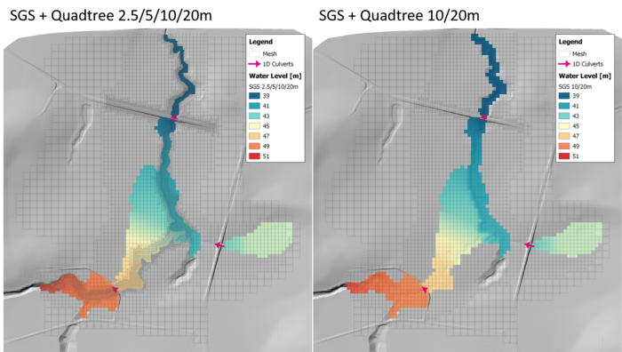
Figure 1 Water level simulation results with SGS. Left: 2.5/5/10/20m Quadtree model. Right: 10/20m Quadtree model.
On the other hand, the same model running without SGS applied creates notably different results in the distance of water travelled and the area of inundation on the floodplain due to the poor topographic representation (one elevation per cell centre and cell face).
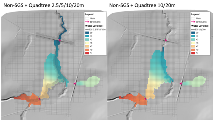
Figure 2 Water level simulation results without SGS. Left: 2.5/5/10/20m Quadtree model. Right: 10/20m Quadtree model.
These examples show how the mesh size sensitivity are significantly reduced if using TUFLOW's implementation of SGS. Therefore, modellers can confidently use a coarser mesh at areas away from the area of interest without adversely affecting the results. However, this has created a challenge on how to map results in areas of coarser mesh. For example, the images below show that whilst the 10/20m mesh and the 2.5/5/10/20m mesh SGS models produce similar water levels, the depth output is much 'smoother' in the 2.5/5/10/20m model due to the finer computational mesh.
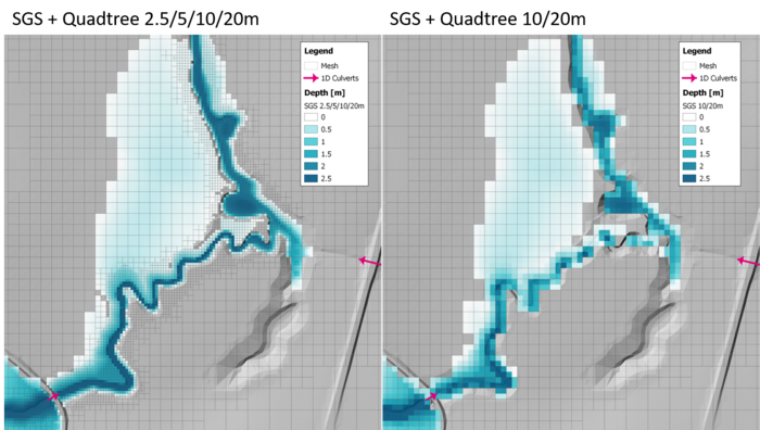
Figure 3 Water depth simulation results with SGS. Left: 2.5/5/10/20m Quadtree model. Right: 10/20m Quadtree model.
In TUFLOW, the depth output is interpolated from the depths at the nearest cell centre and cell corners surrounding the output grid. Because TUFLOW currently doesn't store the underlying high resolution DEM values other than those needed for the SGS hydraulic computations, the interpolated depth may not perfectly represent the actual depth as illustrated in the figure below.
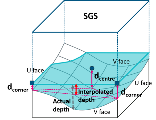
Figure 4 TIN interpolation used for water depth map output with SGS.
This page introduces how to use the ASC_to_ASC remap function, and discusses limitations of the method.
Remapping Water Level to a Finer DEM
The remap function in ASC_to_ASC remaps a TUFLOW water level grid to a high resolution DEM using TIN interpolation. The output is a high resolution water level grid and a high resolution depth grid.
asc_to_asc.exe -remap -wl lowres_h.asc -dem DEM_highres.asc
where:
"-wl <wl_file>"
sets the coarser resolution water level grid to use for the remap.
"-dem <dem_file>"
sets the finer resolution DEM.
The first image below shows the remapped water depth on top of the 10/20m model water level output, and compares it with the original water depth output in the second image. As can be seen, much smooth water depths along the gully and the flood fringes are produced.
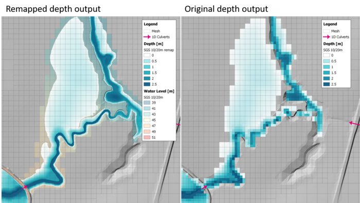
Figure 5 Remapped vs original water depth for 10/20m mesh SGS model.
The next example presents the water level output and the remapped depth output from a flood model using SGS with the buildings included in the DEM. As can be seen in the first image, large portions of the smaller buildings appear submerged by the SGS water level output due to the cells containing these buildings being partially wet. However, the remapped depths (second image) clearly shows the buildings and produces a much higher resolution flood map.
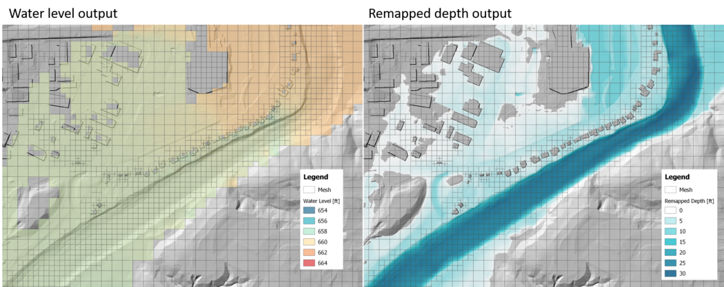
Figure 6 Water level output and remapped water depth in a river flood model.
Remapping of Other Map Output Grids
The utility can also remap additional map output grids (e.g. velocity, hazard and others) to the resolution of the DEM file.
asc_to_asc.exe -remap -wl lowres_h.asc -dem DEM_highres.asc lowres_v.asc lowres_hazard.asc
This command reads in an additional grids 'lowres_v.asc' and 'lowres_hazard.asc' and remaps it to the finer DEM resolution. The figure below compares the original and the remapped hazard outputs from the 10/20m SGS model.
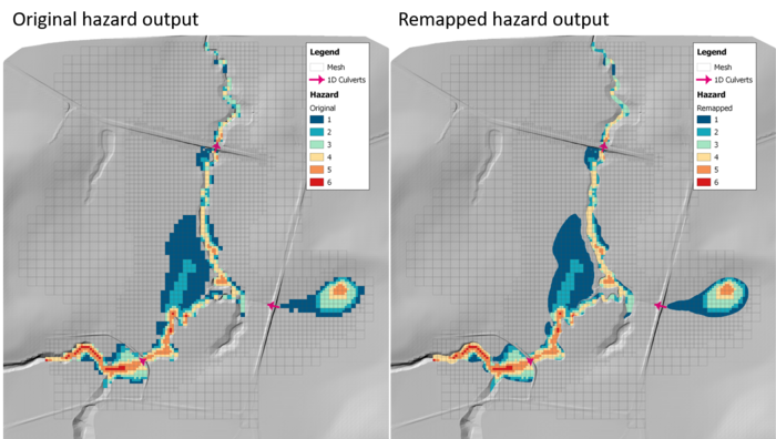
Figure 7 Original vs remapped hazard output for 10/20m mesh SGS model.
It is important to note that, for any output types other than depth, this utility does NOT interpolate the result from the coarser grid to the finer grid, but only extends/reduces the output extent to the dry/wet extent. Therefore, the detail of the remapped hazard above remains the same as the original output grid. The interpolation is not carried out for the following reasons:
- Hazard categories are usually dependent on both water depth and velocity, and it is problematic to interpolate/extrapolate the computed cell averaged velocity to sub-cell scale velocities with varying water depth.
- Should a higher output resolution be required for outputs utilising velocity, a finer mesh in the area should be used.
The figure below shows the hazard output from the 2.5/5/10/20m model, and as can be seen the hazard result is much smoother and more accurate along the gully where the finer cell sizes occur.
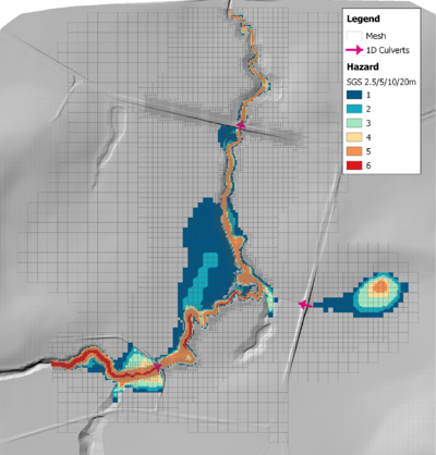
Figure 8 Original hazard output for 2.5/5/10/20m mesh SGS model.
Tip: multiple file names or wildcard are allowed for the extra grid files for remapping.
Model Mesh Size vs Remap Result
Beside the quality of velocity based outputs discussed above, the model mesh size can also impact the remapped output at locations with steep slope as discussed below.
Road Crests
When water flows over a road crest, the remapped water depth may become negative if the output grid size is coarse. The figure below shows the remapped depth over a road crest from models with mesh sizes ranging from 5m to 1.25m. As can be seen, some areas don't have remapped depths despite the water clearly over-topping the road.
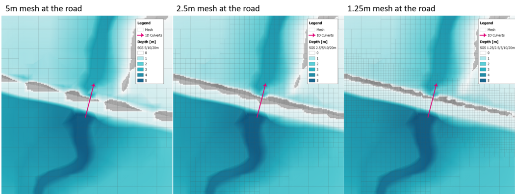
Figure 9 Remapped depths over a road crest from models of different mesh resolutions.
As illustrated in the chart below, the DEM has a much finer resolution and the elevation changes rapidly across the road crest, so when interpolating a coarser water level grid to the finer DEM, the interpolated water level may become lower than the local DEM level. In the 2D solver, this type of location is treated as upstream controlled weir flow with the upstream depth used for the calculation. However, the information that the flow is upstream controlled is not known when remapping, hence the appearance of dry patches on the downstream face of the road crest.
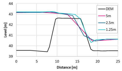
Figure 10 Modelled water level line over the road crest.
Steep Catchments
In direct rainfall models, substantial benefits are being realised from applying SGS. The cell faces now correctly capture the lowest elevations along the gullies to preserve the sub-cell scale flow paths, which can significantly improve the hydrologic response for a whole catchment model (see Duncan Kitts' LinkedIn post: https://www.linkedin.com/pulse/sub-grid-sampling-step-change-way-we-create-apply-hydraulic-kitts/). However, if the cell size becomes too large in areas of significant topographic change, only a small portion of the cell may be wet. This makes the depth plotting extremely challenging and the remapped depth may become negative even though water is flowing through the cell. The blue contour below shows the remapped water depth of a 60m mesh direct rainfall model. As can be seen the flow paths are not continuous along some valleys. The remapped water depth from a 20m mesh model is also plotted as the pink contours underneath the 60m result demonstrating that how the flow paths have become clearer as the mesh size is refined even though the results from these two models are very similar when using SGS.
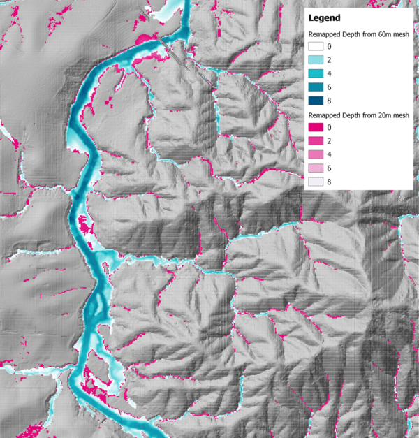
Figure 11 Remapped depth at upstream catchment from different mesh size models.
Conclusion
The benefits of using the combination of Quadtree mesh and Sub-grid Sampling method are many. In this page we focused on the ability of representing the sub-grid scale geometry by SGS method, which allows the user to apply a coarser mesh to reduce the total simulation time without adversely affecting the results. However, the interpolation of map output from a coarser mesh can be challenging as illustrated in the examples above. While we are developing a high resolution output feature within TUFLOW to tackle this issue, the new remapping functions of the ASC_to_ASC utility can be used to post process water level outputs to high resolution depth results. This produces smooth depth output along main flow paths and flood fringes. However, the SGS method and remapping tool is not a panacea, and a computational mesh with sufficient resolution is still needed to produce reasonable and meaningful simulation results, especially where high resolution velocity based map outputs are needed.
Tip: Run your model once with small cell size in a test mode (-t) to produce DEM_Z with all topography modifications with the same resolution as the original DEM for use in the TUFLOW Remapping function.
Finally, should you have some interesting results using SGS, Quadtree or the remapping feature that you would like to share with the TUFLOW community, please feel free to email support@tuflow.com.