TUFLOW 2D Cell Size Selection: Difference between revisions
Chris Huxley (talk | contribs) |
Anne.Kolega (talk | contribs) →Test Case 2 - Results: i.e. |
||
| (62 intermediate revisions by 3 users not shown) | |||
| Line 1: | Line 1: | ||
This page is currently under construction. |
|||
| ⚫ | |||
| ⚫ | |||
=Introduction= |
=Introduction= |
||
This page of the TUFLOW Wiki discusses 2D cell size convergence. |
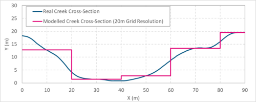
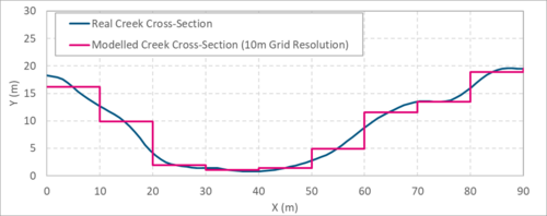
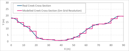
This page of the TUFLOW Wiki discusses 2D cell size convergence. In well designed modelling software such as TUFLOW, cell size convergence refers to the tendency for model results to trend towards a common answer as cell size decreases. This behaviour occurs due to topographic features that influence the hydraulic flow behaviour better approximating reality as resolution increases. The series of creek cross-section images below demonstrate this. As model resolution increases from 20m to 5m the modelled topography progressively matches the real-world geometry more closely.<br> |
||
[[File:Mesh_Converge_XS_20m.png|500px]][[File:Mesh_Converge_XS_10m.png|500px]][[File:Mesh_Converge_XS_05m.png|500px]]<br> |
[[File:Mesh_Converge_XS_20m.png|500px]][[File:Mesh_Converge_XS_10m.png|500px]][[File:Mesh_Converge_XS_05m.png|500px]]<br> |
||
Unfortunately it isn't practical for all models to be designed at an infinitely fine resolution due to the impact it has on simulation speed. Increasing a model resolution will make a simulation run slower. As a rule of thumb, halving the cell size in a model will typically increase the simulation run time by a factor 8. This is due to the number of cells increasing by a factor of (4) four and the necessity for a calculation timestep half that of the larger resolution, translating to (2) twice the number of calculations (4 x 2 = 8). <br> |
|||
The challenge for modellers is |
Whilst high resolution modelling is always desirable, unfortunately it isn't practical in all situations due to the impact increasing resolution has on simulation speed. Increasing resolution, increases the computation load and therfore makes a model run slower. Even though TUFLOW with GPU hardware technology is arguably the fastest simulation software available, the time it takes for a model to run is still an important consideration. The challenge for modellers is knowing what resolution is necessary to achieve results that are fit for purpose with sufficient accuracy whilst also having a run time that's practical (i.e. hours, not days). <br> |
||
<u>[https://tuflow.com/download/Australian_Rainfall_Runoff_Project15_TwoDimensional_Modelling_DraftReport.pdf Australian Rainfall and Runoff |
<u>[https://tuflow.com/download/Australian_Rainfall_Runoff_Project15_TwoDimensional_Modelling_DraftReport.pdf Australian Rainfall and Runoff - Two Dimensional Modelling in Urban and Rural Floodplain Guideline]</u> provides some recommendations on this topic. It states: <br> |
||
: ''The resolution of a 2D model grid/mesh determines the scale of physical features and flow behaviour that can be modelled for a given study area. Selection of an appropriate resolution is generally driven by a combination of the following factors: <br> |
: ''The resolution of a 2D model grid/mesh determines the scale of physical features and flow behaviour that can be modelled for a given study area. Selection of an appropriate resolution is generally driven by a combination of the following factors: <br> |
||
: ''* The scale of topographic and/or flow phenomena to be modelled |
: ''* The scale of topographic and/or flow phenomena to be modelled |
||
| Line 34: | Line 30: | ||
This Wiki page uses two test cases to discuss this topic. Quantitative results are presented demonstrating how and when resolution assumptions have a tangible impact on model results. TUFLOW HPC and it's GPU Module have been used for all simulations documented in the following sections. The computer used for the modelling has a NVIDIA GeForce GTX 1080 Ti GPU card. |
This Wiki page uses two test cases to discuss this topic. Quantitative results are presented demonstrating how and when resolution assumptions have a tangible impact on model results. TUFLOW HPC and it's GPU Module have been used for all simulations documented in the following sections. The computer used for the modelling has a NVIDIA GeForce GTX 1080 Ti GPU card. |
||
=Webinar Link= |
|||
| ⚫ | |||
A webinar was recorded that summarises the written content below. It is hosted on <u>[https://www.youtube.com/watch?v=dZWpnKZBKJk&feature=youtu.be YouTube]</u> or available via our <u>[[TUFLOW_Modelling_Webinar | Webinar Page]]</u>. |
|||
| ⚫ | This test case has been sourced from the <u>[https://www.tuflow.com/Download/Publications/UK%20EA%202D%20Benchmarking%20Results.TUFLOW%20Products%202017-09.pdf UK Environment Agency 2D Hydraulic Model Benchmark Test dataset]</u>. It is referred to as Test 5 in the Environment Agency (EA) |
||
| ⚫ | |||
| ⚫ | This test case has been sourced from the <u>[https://www.tuflow.com/Download/Publications/UK%20EA%202D%20Benchmarking%20Results.TUFLOW%20Products%202017-09.pdf UK Environment Agency 2D Hydraulic Model Benchmark Test dataset]</u>. It is referred to as Test 5 in the Environment Agency (EA) document. The EA designed this test to simulate flood wave propagation down a river valley following the failure of a dam. The valley DEM is ~0.8 km by ~17 km and the valley slopes downstream on a slope of ~0.01 in its upper region, easing to ~0.001 at lower elevations. The model uses a single manning's n value of 0.04 across the entire domain. |
||
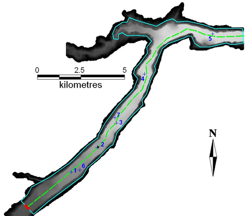
The model topography and EA reporting points are shown below. <br> |
The model topography and EA reporting points are shown below. <br> |
||
[[File:Mesh_Converge_Model_Description_001.png|500px]] |
[[File:Mesh_Converge_Model_Description_001.png|500px]] |
||
| Line 42: | Line 41: | ||
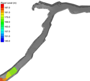
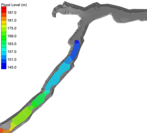
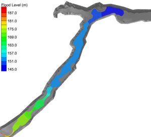
The model has a single inflow at the top of the catchment. The inflow hydrograph that has been used is shown below. Although the inflow only introduces water into the model for 100 minutes the model has been run for a simulation period of 30 hours. This was a requirement in the original EA model benchmark documentation. <br> |
The model has a single inflow at the top of the catchment. The inflow hydrograph that has been used is shown below. Although the inflow only introduces water into the model for 100 minutes the model has been run for a simulation period of 30 hours. This was a requirement in the original EA model benchmark documentation. <br> |
||
[[File:Mesh Converge Model Inflow 001.png|500px]]<br> |
[[File:Mesh Converge Model Inflow 001.png|500px]]<br> |
||
{| class="wikitable " |
|||
[[File:Mesh_Converge_SMS_0.5hr.png|300px]][[File:Mesh_Converge_SMS_1.5hr.png|300px]][[File:Mesh_Converge_SMS_2.5hr.png|300px]][[File:Mesh_Converge_SMS_4hr.png|300px]] |
| [[File:Mesh_Converge_SMS_0.5hr.png|300px]] || [[File:Mesh_Converge_SMS_1.5hr.png|300px]] || [[File:Mesh_Converge_SMS_2.5hr.png|300px]] ||[[File:Mesh_Converge_SMS_4hr.png|300px]] |
||
|- |
|||
| t = 0.5h || t = 1.5h || t = 2.5h || t = 4.0h |
|||
|} |
|||
The EA benchmark testing originally assumed a 50m cell resolution. For the purpose of this assessment a range of cell sizes have been used to determine the impact changing grid resolution has on the model results. The following grid resolutions were used: |
The EA benchmark testing originally assumed a 50m cell resolution. For the purpose of this assessment a range of cell sizes have been used to determine the impact changing grid resolution has on the model results. The following grid resolutions were used: |
||
| Line 62: | Line 65: | ||
| '''Cell Size''' || '''Location 4 Result'''|| '''Location 5 Result''' || '''Mesh Resolution Figure''' |
| '''Cell Size''' || '''Location 4 Result'''|| '''Location 5 Result''' || '''Mesh Resolution Figure''' |
||
|- |
|- |
||
| '''10m''' || [[File:Mesh_Converge_Exg_P4_010.png|500px]] || [[File:Mesh Converge Exg P5 010.png|500px]] ||[[File:Mesh Converge Grid 010.png|500px]] |
| '''10m (33ft)''' || [[File:Mesh_Converge_Exg_P4_010.png|500px]] || [[File:Mesh Converge Exg P5 010.png|500px]] ||[[File:Mesh Converge Grid 010.png|500px]] |
||
|- |
|- |
||
| '''20m''' || [[File:Mesh Converge Exg P4 020.png|500px]] || [[File:Mesh Converge Exg P5 020.png|500px]] || [[File:Mesh_Converge_Grid_020.png|500px]] |
| '''20m (66ft)''' || [[File:Mesh Converge Exg P4 020.png|500px]] || [[File:Mesh Converge Exg P5 020.png|500px]] || [[File:Mesh_Converge_Grid_020.png|500px]] |
||
|- |
|- |
||
| '''50m''' || [[File:Mesh Converge Exg P4 050.png|500px]] || [[File:Mesh Converge Exg P5 050.png|500px]] ||[[File:Mesh_Converge_Grid_050.png|500px]] |
| '''50m (164ft)''' || [[File:Mesh Converge Exg P4 050.png|500px]] || [[File:Mesh Converge Exg P5 050.png|500px]] ||[[File:Mesh_Converge_Grid_050.png|500px]] |
||
|- |
|- |
||
| '''100m''' || [[File:Mesh Converge Exg P4 100.png|500px]]|| [[File:Mesh Converge Exg P5 100.png|500px]] || [[File:Mesh Converge Grid 100.png|500px]] |
| '''100m (328ft)''' || [[File:Mesh Converge Exg P4 100.png|500px]]|| [[File:Mesh Converge Exg P5 100.png|500px]] || [[File:Mesh Converge Grid 100.png|500px]] |
||
|- |
|- |
||
| '''150m''' || [[File:Mesh Converge Exg P4 150.png|500px]] || [[File:Mesh Converge Exg P5 150.png|500px]] ||[[File:Mesh Converge Grid 150.png|500px]] |
| '''150m (492ft)''' || [[File:Mesh Converge Exg P4 150.png|500px]] || [[File:Mesh Converge Exg P5 150.png|500px]] ||[[File:Mesh Converge Grid 150.png|500px]] |
||
|- |
|- |
||
| '''200m''' || [[File:Mesh Converge Exg P4 200.png|500px]] || [[File:Mesh Converge Exg P5 200.png|500px]] ||[[File:Mesh Converge Grid 200.png|500px]] |
| '''200m (656ft)''' || [[File:Mesh Converge Exg P4 200.png|500px]] || [[File:Mesh Converge Exg P5 200.png|500px]] ||[[File:Mesh Converge Grid 200.png|500px]] |
||
|- |
|- |
||
| '''250m''' || [[File:Mesh Converge Exg P4 250.png|500px]] || [[File:Mesh Converge Exg P5 250.png|500px]] ||[[File:Mesh Converge Grid 250.png|500px]] |
| '''250m (820ft)''' || [[File:Mesh Converge Exg P4 250.png|500px]] || [[File:Mesh Converge Exg P5 250.png|500px]] ||[[File:Mesh Converge Grid 250.png|500px]] |
||
|} |
|} |
||
== Test Case 1 - Discussion == |
== Test Case 1 - Discussion == |
||
The graphed results indicate convergence is observed for all cases with a cell resolution equal to or less than 100m. The grid figures presented to the right of the graphs suggest the 100m cell resolution case has approximately (4) four cells laterally across the valley that the dam break flow is contained within. Although the 400-600m wide valley isn't a traditional creek or river channel, the scale of flow associated with the dam break means the valley is behaving like one. Minor topographic features within the valley are too small to have a significant impact on the flood behaviour for flow conditions of this large magnitude. This result trend is consistent with the Australian Rainfall and Runoff (ARR) cell size recommendation for the flow in a channel, "In order to adequately resolve flow in a channel it is desirable to provide at least 5 grid/mesh elements laterally across the channel". |
The graphed results indicate convergence is observed for all cases with a cell resolution equal to or less than 100m (328ft). The grid figures presented to the right of the graphs suggest the 100m cell resolution case has approximately (4) four cells laterally across the valley that the dam break flow is contained within. Although the 400-600m (1,300ft - 2000ft) wide valley isn't a traditional creek or river channel, the scale of flow associated with the dam break means the valley is behaving like one. Minor topographic features within the valley are too small to have a significant impact on the flood behaviour for flow conditions of this large magnitude. This result trend is consistent with the Australian Rainfall and Runoff (ARR) cell size recommendation for the flow in a channel, "In order to adequately resolve flow in a channel it is desirable to provide at least 5 grid/mesh elements laterally across the channel". |
||
Simulation time can influence model resolution selection. This is not the case in this situation. All models have run in under 5 minutes using TUFLOW HPC's GPU hardware module. |
Simulation time can influence model resolution selection. This is not the case in this situation. All models have run in under 5 minutes using TUFLOW HPC's GPU hardware module. |
||
| Line 84: | Line 87: | ||
{| class="wikitable " |
{| class="wikitable " |
||
| '''Cell Size''' || '''Model Size <br> (Cell Count)'''|| '''Simulation Run Time <br> (seconds)''' || '''Judgement of Convergence <br> (Yes / No)''' |
| '''Cell Size''' || '''Model Size <br> (Cell Count)'''|| '''Simulation Run Time <br> (seconds)''' || '''Judgement of Convergence <br> (Yes / No)''' || '''Required GPU Memory <br> (GB)''' |
||
|- |
|- |
||
| 10m (33ft) || 188,240 || 284 || Yes |
| 10m (33ft) || 188,240 || 284 || Yes || 0.15 |
||
|- |
|- |
||
| 20m (66ft) || 47,080 || 98 || Yes |
| 20m (66ft) || 47,080 || 98 || Yes || 0.04 |
||
|- |
|- |
||
| 50m (164ft) || 7,540 || 32 || Yes |
| 50m (164ft) || 7,540 || 32 || Yes || 0.01 |
||
|- |
|- |
||
| 100m (328ft) || 1,880 || 15 || Yes |
| 100m (328ft) || 1,880 || 15 || Yes || <0.01 |
||
|- |
|- |
||
| 150m (492ft) || 840 || 10 || No |
| 150m (492ft) || 840 || 10 || No || <0.01 |
||
|- |
|- |
||
| 200m (656ft) || 480 || 9 || No |
| 200m (656ft) || 480 || 9 || No || <0.01 |
||
|- |
|- |
||
| 250m (820ft) || 300 || 7 || No |
| 250m (820ft) || 300 || 7 || No || <0.01 |
||
|} |
|} |
||
Since simulation time is not a limiting factor in this case selection of cell size only needs to consider the result accuracy. What is appropriate in terms of accuracy is influenced by the intended use of the model. For example, if lot scale assessment of inundation and structural damage risk is required, selection of the 10m cell size may be appropriate. Alternatively, if the model is only intended to inform broad-scale risk, the 50m or 100m cell size may be sufficient. |
Since simulation time is not a limiting factor in this case, selection of cell size only needs to consider the result accuracy. What is appropriate in terms of accuracy is influenced by the intended use of the model. For example, if lot scale assessment of inundation and structural damage risk is required, selection of the 10m (33ft) cell size may be appropriate to provide high resolution mapping of the velocity gradients. Alternatively, if the model is only intended to inform broad-scale inundation risk, the 50m (164ft) or 100m (328ft) cell size may be sufficient. |
||
= Test Case 2 - Urbanised Catchment = |
= Test Case 2 - Urbanised Catchment (USA) = |
||
This test case uses a hypothetical urban model. The model encompasses the entire catchment and covers an area of approximately |
This test case uses a hypothetical urban model. The model encompasses the entire catchment and covers an area of approximately 21 square miles (54 square kilometres). Development within the catchment ranges from rural undeveloped in the mountainous upper catchment to dense urban development in the lower catchment. <br> |
||
[[File:Mesh Converge Direct Rainfall Topo.png| |
[[File:Mesh Converge Direct Rainfall Topo.png|700px]][[File:Mesh Converge Direct Rainfall Manning n.png|700px]]<br> |
||
A direct rainfall approach has been used, applying rainfall directly to every cell within the model. The event hyetograph is a hypothetical 24 hour extreme event. The simulation duration has also been set to 24 hours.<br> |
A direct rainfall approach has been used, applying rainfall directly to every cell within the model. The event hyetograph is a hypothetical 24 hour extreme event. The simulation duration has also been set to 24 hours.<br> |
||
''Note, if you are unfamiliar with the direct rainfall modelling approach, this <u>[https://www.tuflow.com/Download/Publications/HWRS2016_Huxley_Paper.pdf Hydrology and Water Symposium]</u> paper introduces the concept.'' <br> |
''Note, if you are unfamiliar with the direct rainfall modelling approach, this <u>[https://www.tuflow.com/Download/Publications/HWRS2016_Huxley_Paper.pdf Hydrology and Water Symposium]</u> paper introduces the concept.'' <br> |
||
[[File:Mesh_Converge_Direct_Hyetograph.png|700px]]<br> |
|||
'''Image of Rainfall Hyetograph '''<br> |
|||
The following grid resolutions were used to test the impact of cell size on the assessment results and simulation time:<br> |
The following grid resolutions were used to test the impact of cell size on the assessment results and simulation time:<br> |
||
* 10ft (3.0m) resolution |
* 10ft (3.0m) cell resolution – 5,821,533 total cell count |
||
* |
* 12ft (3.7m) cell resolution – 4,042,960 total cell count |
||
* 15ft (4.6m) resolution – 2,587,629 cell count |
* 15ft (4.6m) cell resolution – 2,587,629 total cell count |
||
* 20ft (6.1m) resolution – 1,455,869 cell count |
* 20ft (6.1m) cell resolution – 1,455,869 total cell count |
||
* |
*30ft (9.1m) cell resolution – 647,003 total cell count |
||
* 50ft (15.2m) cell resolution – 232,957 total cell count |
|||
* 75ft (22.9m) cell resolution – 103,525 total cell count |
|||
Since the direct rainfall modelling approach means the entire model is "wet", output has been filtered to only show results in locations where the flood depth exceeds 0.3ft. This is done in TUFLOW using the TCF command "Map Cutoff Depth == ". |
|||
== Test Case 2 - Results == |
== Test Case 2 - Results == |
||
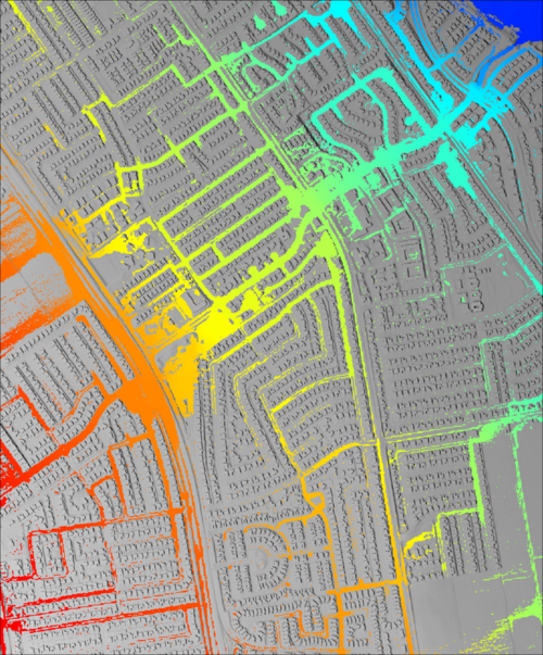
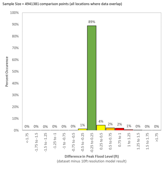
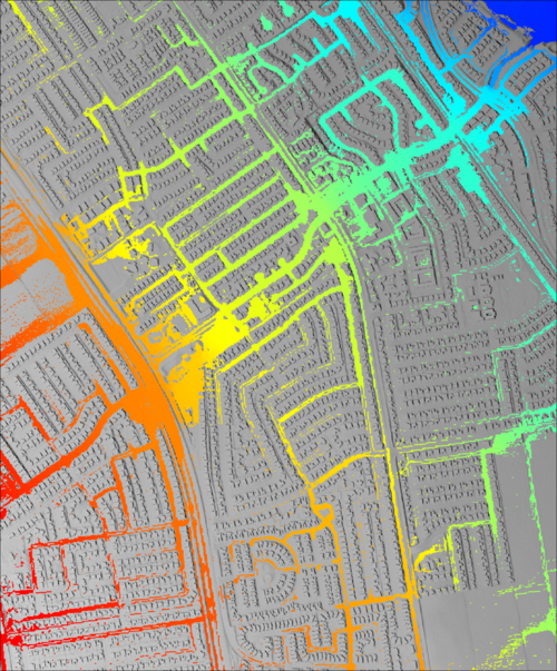
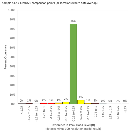
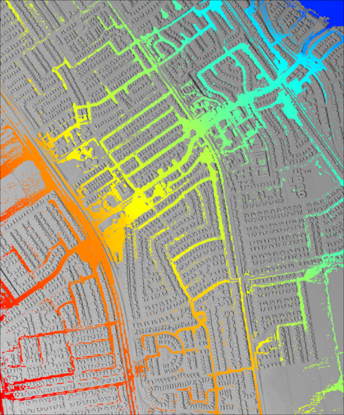
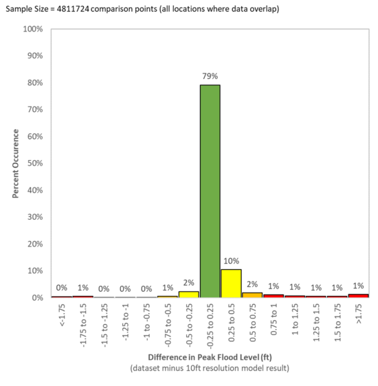
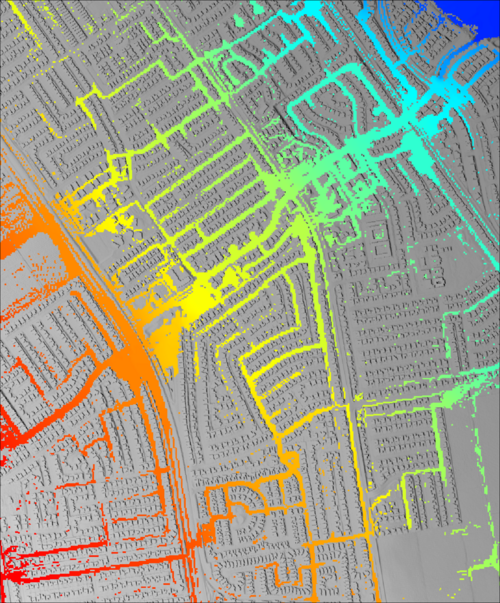
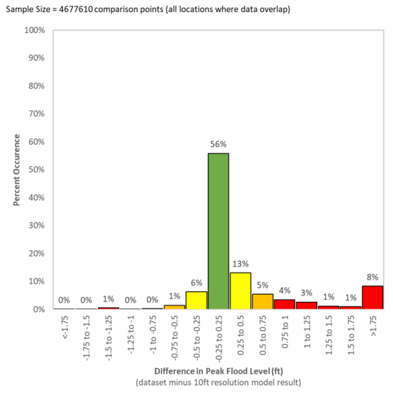
The cell convergence test results are summarised in the table below. They have been presented in a histogram form. The histograms are calculated by subtracting the peak (maximum) flood level result raster grid for the larger cell resolution simulation from the 10ft cell resolution result. The result difference has been sampled at every pixel in the raster datasets where flood information is present in both result files (i.e. they overlap).<br> |
|||
{| class="wikitable " |
{| class="wikitable " |
||
| '''Cell Resolution, Model Size and Simulation Run Time''' |
| '''Cell Resolution, Model Size <br> and Simulation Run Time''' || '''Difference in Water Level Result (ft)''' <br> (Relative to 10ft Resolution Model)<br> (Agreement Scale: Green = Excellent, Yellow = Good, Orange = Average, Red = Poor) || '''Sample Peak (Maximum) Water Level Result''' |
||
|- |
|- |
||
| '''10ft (3.0m) cell size <br> |
| '''10ft (3.0m) cell size <br><br>5,821,533 total cell count<br><br> 9.2hr simulation run time'''||N/A <br><br>The histogram graphs below are calculated by subtracting <br>the peak (maximum) flood level result from the 10ft cell <br>resolution peak (maximum) flood level result <br>(shown to the right) || [[File:Mesh_Converge_Direct_Rainfall_10ft_002.png|500px]] |
||
|- |
|- |
||
| ''' |
| '''12ft (3.7m) cell size<br><br>4,042,960 total cell count<br><br> 7.5hr simulation run time'''||[[File:Mesh_Converge_Direct_Rainfall_12ft_HIST.png|550px]] || [[File:Mesh_Converge_Direct_Rainfall_12ft_002.png|500px]] |
||
|- |
|- |
||
| '''15ft (4.6m) cell size<br> |
| '''15ft (4.6m) cell size<br><br>2,587,629 total cell count<br><br> 4.4hr simulation run time'''||[[File:Mesh_Converge_Direct_Rainfall_15ft_HIST.png|550px]] || [[File:Mesh_Converge_Direct_Rainfall_15ft_002.png|500px]] |
||
|- |
|- |
||
| '''20ft (6.1m) cell size<br> |
| '''20ft (6.1m) cell size<br><br>1,455,869 total cell count<br><br> 1.8hr simulation run time'''|| [[File:Mesh_Converge_Direct_Rainfall_20ft_HIST.png|550px]] || [[File:Mesh_Converge_Direct_Rainfall_20ft_002.png|500px]] |
||
|- |
|- |
||
| '''30ft (9.1m) cell size<br> |
| '''30ft (9.1m) cell size<br><br>647,003 total cell count<br><br> 0.65hr simulation run time'''|| [[File:Mesh_Converge_Direct_Rainfall_30ft_HIST.png|550px]] || [[File:Mesh_Converge_Direct_Rainfall_30ft_002.png|500px]] |
||
|- |
|- |
||
| '''50ft (15.2m) cell size<br>232,957 cell count<br> 0. |
| '''50ft (15.2m) cell size<br><br>232,957 total cell count<br><br> 0.23hr simulation run time''' ||[[File:Mesh_Converge_Direct_Rainfall_50ft_HIST.png|550px]] || [[File:Mesh Converge Direct Rainfall 50ft 002.png|500px]] |
||
|- |
|||
| '''75ft (22.9m) cell size<br><br>103,525 total cell count<br><br> 0.08hr simulation run time''' ||[[File:Mesh_Converge_Direct_Rainfall_75ft_HIST.png|550px]] || [[File:Mesh Converge Direct Rainfall 75ft 002.png|500px]] |
|||
|} |
|} |
||
== Test Case 2 - Discussion== |
== Test Case 2 - Discussion== |
||
The urban model testing indicates result convergence occurs when the cell resolution is less than 20ft. This observation agrees with the ARR guideline recommendation for urban models to use a cell resolution of |
|||
2m (6.6ft) to 5m (16.4ft). <br> |
|||
{| class="wikitable " |
|||
| '''Cell Size''' || '''Model Size <br> (Cell Count)'''|| '''Simulation Run Time <br> (hours)''' || '''Judgement of Convergence <br> (Yes / No)''' || '''Required GPU Memory <br> (GB) |
|||
|- |
|||
| 10ft (3.0m) || 5,821,533 || 9.2hr || Yes || 1.74 |
|||
|- |
|||
| 12ft (3.7m) || 4,042,960 || 7.5hr || Yes || 1.20 |
|||
|- |
|||
| 15ft (4.6m) || 2,587,629 || 4.4hr || Yes || 0.77 |
|||
|- |
|||
| 20ft (6.1m) || 1,455,869 || 1.8hr || Yes || 0.44 |
|||
|- |
|||
| 30ft (9.1m) || 647,003 || 0.65hr || Mostly || 0.20 |
|||
|- |
|||
| 50ft (15.2m) || 232,957 || 0.23hr || No || 0.07 |
|||
|- |
|||
| 75ft (22.9m) || 103,525 || 0.08hr || No || 0.03 |
|||
|} |
|||
As per Test Case 1, selection of the appropriate cell resolution during a real-world project requires consideration of the intended use of the results and also how the simulation run time impacts the overall project timeline. |
|||
* Detailed integrated 1D/2D urban modelling may adopt the 15ft (4.6m) or slightly finer 12ft (3.7m) cell resolution if the cumulative simulation time for all model events/scenarios does not adversely impact the project timeline. This timeframe consideration is particularly relevant in locations such as Australia where an ensemble methodology is currently replacing single event approaches as a way to address uncertainty associated with hydrologic assumptions. |
|||
* Broad-scale quick run simulation for urban flood forecasting purposes may adopt a coarser 20ft cell resolution or investigate the suitability of a 25ft cell resolution to achieve a quicker simulation turnaround time.<br> |
|||
= Common Questions Answered (FAQ)= |
|||
==How much will my runtime change when changing cell size?== |
|||
Solution time for a model is dependent on a number of factors: the solution scheme used, the size and duration of the model, the nature of the hydraulics within the model, the model features selected, and the hardware that it is executed on. However, once a model is developed at a relatively coarse resolution, there are some guidelines that can assist with predicting what the solve time will be as the resolution is refined. These can be useful for estimating whether the refined model will run overnight or need a few days.<br> |
|||
TUFLOW classic uses an implicit solution scheme that sweeps along columns and rows of cells. The solution scheme is one of the most efficient ever devised for solving the Shallow Water Equations (SWEs), but cannot be parallelised as the order of calculations are not independent. As a result the code is written to execute on a single core of a CPU. The time required to solve a model is almost exactly proportional to the number of wet cells in the model and the number of timesteps required. When the model cell size is halved, the number of cells increases by a factor of 4, and the timestep reduces by a factor of 2, so the model solve time increases by very close to a factor of 8.<br> |
|||
TUFLOW HPC uses an explicit solution scheme, for which the cell-based calculations are able to be performed in parallel. This can be done using multiple cores of the CPU, but it is more efficiently done using the many thousands of cores of modern GPUs. The model is cut into small tiles that are divided up amongst the streaming multi-controllers (SMs) of the GPU, with each SM distributing the cell calculations of its tile amongst its cores. However, there are still some calculations that must be done at the ‘top-level’ of the model, such as updating boundary flows and levels, extracting the plot output data, timestep control, and the process of configuring and launching the GPU parallel code. These tasks remain on the CPU and cannot be parallelised as the order of execution of these instructions is vitally important. So the overall model execution contains a mix of both parallel and serial work, with the total model solve time being the sum of both. As a result, the solve time for a model doesn’t follow a simple scaling rule. The cell-based component is still proportional to the number of cells times the number of timesteps, whereas the serial component of the work is generally only proportional to the number of timesteps. To be correct, this was also true of the single core solver for TUFLOW classic, but because the cell-based component was generally more than 99% of the work load, the scaling followed the simple rule of 8 times longer for half the cell size.<br> |
|||
In summary, for small models running with TUFLOW HPC, the solution time will increase by a factor somewhere in the range of 3 to 8 for a halving of the cell size. Once the model is sufficiently large that the cell-based calculations (running in parallel on the GPU) are taking most of the time, the time increase factor becomes close to 8. Exactly what is a “large” model will depend of the relative speed of the GPU and CPU. For that latest GPUS (as of 2021 this means the Nvidia A100 and RTX 30xx series) large typically means well over a million cells.<br> |
|||
However, there is one last and important caveat when refining cell size. The explicit algorithm used by TUFLOW HPC requires that the timestep is also subject to Peclet (diffusion) number control, not just Courant (velocity) number control. As Peclet number is inversely proportional to cell size squared, whereas Courant number is just inversely proportional to cell size, the model will transition from Courant number control to Peclet number control once the cell size becomes small enough. This means that the factor of 8 on time for a halving of cell size will eventually become a factor of 16. This was not a feature of TUFLOW Classic. In general, we do not recommend refining cell size well into the region where timestep control is completely dominated by the Peclet number (the Nd column in the HPC output). The flows in the primary channels are usually well converged by this point, and the 2D map outputs may not reveal a lot of additional detail in the velocity fields.<br> |
|||
| ⚫ | |||
| ⚫ | |||
{{Tips Navigation |
|||
|uplink=[[ TUFLOW_Modelling_Guidance | Back to TUFLOW Modelling Guidance]] |
|||
}} |
|||
Latest revision as of 12:07, 2 April 2026
Introduction
This page of the TUFLOW Wiki discusses 2D cell size convergence. In well designed modelling software such as TUFLOW, cell size convergence refers to the tendency for model results to trend towards a common answer as cell size decreases. This behaviour occurs due to topographic features that influence the hydraulic flow behaviour better approximating reality as resolution increases. The series of creek cross-section images below demonstrate this. As model resolution increases from 20m to 5m the modelled topography progressively matches the real-world geometry more closely.
Whilst high resolution modelling is always desirable, unfortunately it isn't practical in all situations due to the impact increasing resolution has on simulation speed. Increasing resolution, increases the computation load and therfore makes a model run slower. Even though TUFLOW with GPU hardware technology is arguably the fastest simulation software available, the time it takes for a model to run is still an important consideration. The challenge for modellers is knowing what resolution is necessary to achieve results that are fit for purpose with sufficient accuracy whilst also having a run time that's practical (i.e. hours, not days).
Australian Rainfall and Runoff - Two Dimensional Modelling in Urban and Rural Floodplain Guideline provides some recommendations on this topic. It states:
- The resolution of a 2D model grid/mesh determines the scale of physical features and flow behaviour that can be modelled for a given study area. Selection of an appropriate resolution is generally driven by a combination of the following factors:
- * The scale of topographic and/or flow phenomena to be modelled
- * The desired level of detail to be achieved in the model outputs
- * The length of event time and consequent run time
- * The size of the area of interest
- Details of the model schematisation process including resolution aspects are described in Chapter 6. Chapter 7 also highlights the importance of grid/mesh resolutions in achieving manageable run times to maximise calibration outcomes. Table 10-2 (below) provides guidance on levels of model resolution that may be appropriate in certain typical situations.
| Modelling Case | Typical 2D Cell Resolution |
| Flow in Channel | In order to adequately resolve flow in a channel it is desirable to provide at least 5 grid/mesh elements laterally across the channel |
| Urban Overland | Most urban flood models employ grid/mesh resolutions of 2m to 5m. |
| Flow in Floodplain | Rural floodplain models typically employ grid/mesh resolutions of 10m and 50m (although resolutions up to 200m have been used) depending on the size of the area to be analysed, the characteristics/dimensions of the floodplain and the desired level of output detail. |
| Lakes and Estuaries | These situations often include areas of open water where less detail is required than along the water body boundary. Such situations are well suited to a flexible mesh rather than fixed grid based model as the mesh is able to incorporate a change of resolution across the model domain. Element resolutions for these models can span the full range as described above depending on project requirements. |
| Flow Over and Embankment | Embankments effectively act as weirs in the floodplain context. Many 2D modelling packages have automatic or manually activated corrections that compensate for the error in head loss typically associated with modelling broad-crested weir flow with a 2D scheme. For practical purposes, a single 2D element is generally adequate to represent the impact of a levee, road or railway embankment. The resolution of these elements is generally not a significant limitation on the schematisation of most domains. |
This Wiki page uses two test cases to discuss this topic. Quantitative results are presented demonstrating how and when resolution assumptions have a tangible impact on model results. TUFLOW HPC and it's GPU Module have been used for all simulations documented in the following sections. The computer used for the modelling has a NVIDIA GeForce GTX 1080 Ti GPU card.
Webinar Link
A webinar was recorded that summarises the written content below. It is hosted on YouTube or available via our Webinar Page.
Test Case 1 - Rural Dam Break (United Kingdom)
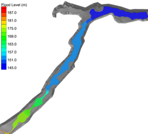
This test case has been sourced from the UK Environment Agency 2D Hydraulic Model Benchmark Test dataset. It is referred to as Test 5 in the Environment Agency (EA) document. The EA designed this test to simulate flood wave propagation down a river valley following the failure of a dam. The valley DEM is ~0.8 km by ~17 km and the valley slopes downstream on a slope of ~0.01 in its upper region, easing to ~0.001 at lower elevations. The model uses a single manning's n value of 0.04 across the entire domain.
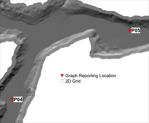
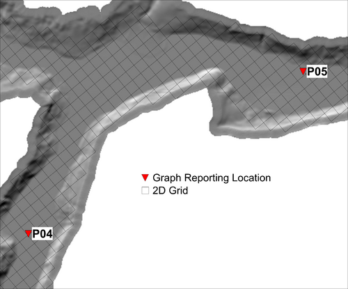
The model topography and EA reporting points are shown below.

The model has a single inflow at the top of the catchment. The inflow hydrograph that has been used is shown below. Although the inflow only introduces water into the model for 100 minutes the model has been run for a simulation period of 30 hours. This was a requirement in the original EA model benchmark documentation.

 |
 |
 |
|
| t = 0.5h | t = 1.5h | t = 2.5h | t = 4.0h |
The EA benchmark testing originally assumed a 50m cell resolution. For the purpose of this assessment a range of cell sizes have been used to determine the impact changing grid resolution has on the model results. The following grid resolutions were used:
- 10m (33ft) resolution - 188,240 cell count
- 20m (66ft) resolution - 47,080 cell count
- 50m (164ft) resolution - 7,540 cell count
- 100m (328ft) resolution - 1,880 cell count
- 150m (492ft) resolution - 840 cell count
- 200m (656ft) resolution - 480 cell count
- 250m (820ft) resolution - 300 cell count
Test Case 1 - Results
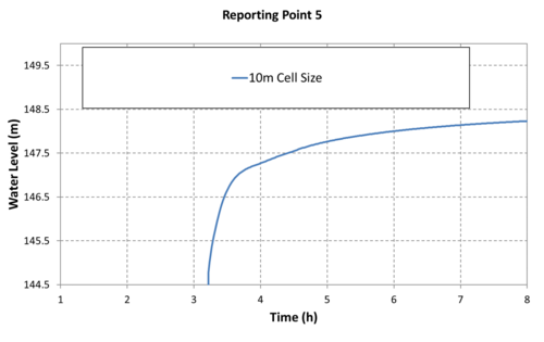
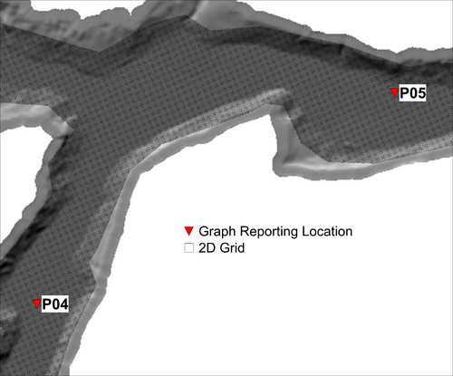
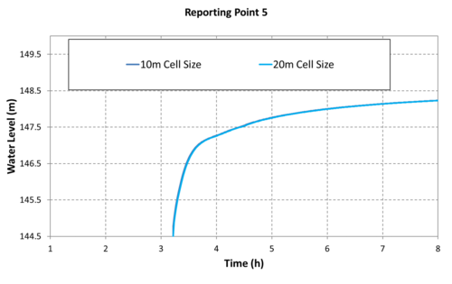
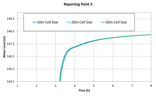
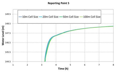
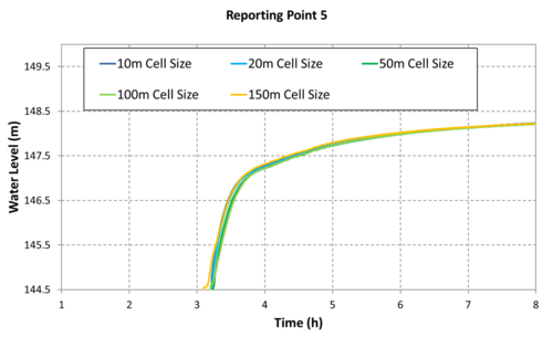
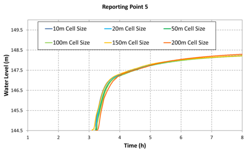
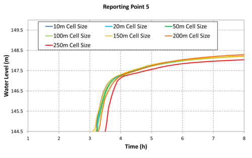
In the interest or keeping this page brief we have focused our result presentation on EA reporting points 4 and 5. Their location furthest downstream in the catchment makes them the most sensitive of all EA 7 reporting points. This is due to any divergence in result caused by poor representation of the upstream topography accumulating, amplifying the result difference associated with a change in cell resolution at these selected locations.
Results are presented below. Although the figures are shown in sequence (from fine to coarse resolution), the results are overlayed on one another moving through the dataset so it is obvious if poor convergence occurs.
| Cell Size | Location 4 Result | Location 5 Result | Mesh Resolution Figure |
| 10m (33ft) | 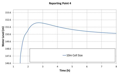 |
 |
|
| 20m (66ft) | 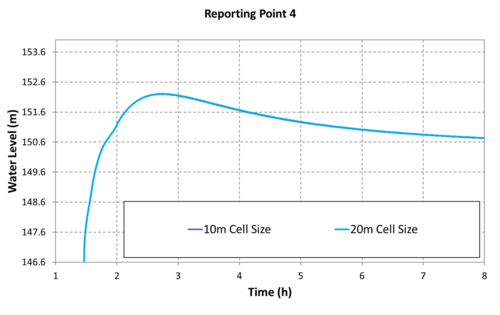 |
 |
|
| 50m (164ft) | 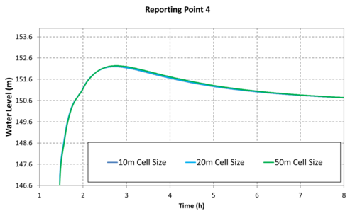 |
 |
|
| 100m (328ft) | 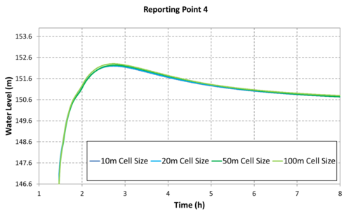 |
 |

|
| 150m (492ft) | 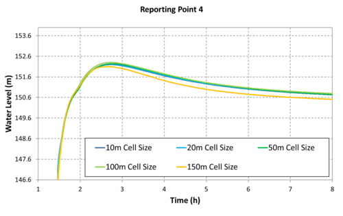 |
 |
|
| 200m (656ft) | 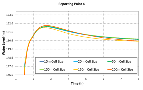 |
 |

|
| 250m (820ft) | 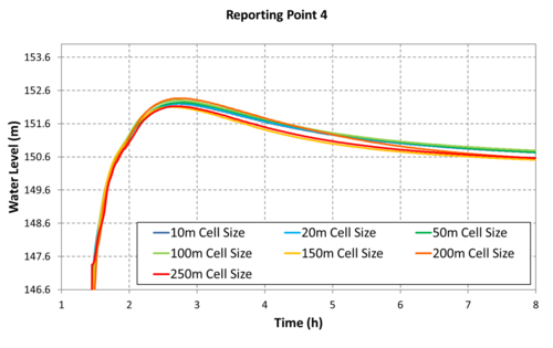 |
 |

|
Test Case 1 - Discussion
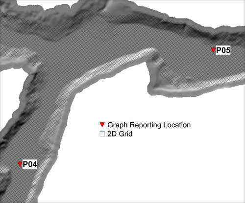
The graphed results indicate convergence is observed for all cases with a cell resolution equal to or less than 100m (328ft). The grid figures presented to the right of the graphs suggest the 100m cell resolution case has approximately (4) four cells laterally across the valley that the dam break flow is contained within. Although the 400-600m (1,300ft - 2000ft) wide valley isn't a traditional creek or river channel, the scale of flow associated with the dam break means the valley is behaving like one. Minor topographic features within the valley are too small to have a significant impact on the flood behaviour for flow conditions of this large magnitude. This result trend is consistent with the Australian Rainfall and Runoff (ARR) cell size recommendation for the flow in a channel, "In order to adequately resolve flow in a channel it is desirable to provide at least 5 grid/mesh elements laterally across the channel".
Simulation time can influence model resolution selection. This is not the case in this situation. All models have run in under 5 minutes using TUFLOW HPC's GPU hardware module.
| Cell Size | Model Size (Cell Count) |
Simulation Run Time (seconds) |
Judgement of Convergence (Yes / No) |
Required GPU Memory (GB) |
| 10m (33ft) | 188,240 | 284 | Yes | 0.15 |
| 20m (66ft) | 47,080 | 98 | Yes | 0.04 |
| 50m (164ft) | 7,540 | 32 | Yes | 0.01 |
| 100m (328ft) | 1,880 | 15 | Yes | <0.01 |
| 150m (492ft) | 840 | 10 | No | <0.01 |
| 200m (656ft) | 480 | 9 | No | <0.01 |
| 250m (820ft) | 300 | 7 | No | <0.01 |
Since simulation time is not a limiting factor in this case, selection of cell size only needs to consider the result accuracy. What is appropriate in terms of accuracy is influenced by the intended use of the model. For example, if lot scale assessment of inundation and structural damage risk is required, selection of the 10m (33ft) cell size may be appropriate to provide high resolution mapping of the velocity gradients. Alternatively, if the model is only intended to inform broad-scale inundation risk, the 50m (164ft) or 100m (328ft) cell size may be sufficient.
Test Case 2 - Urbanised Catchment (USA)
This test case uses a hypothetical urban model. The model encompasses the entire catchment and covers an area of approximately 21 square miles (54 square kilometres). Development within the catchment ranges from rural undeveloped in the mountainous upper catchment to dense urban development in the lower catchment.
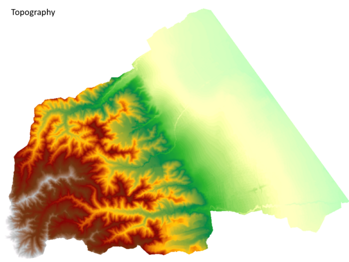
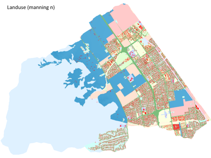
A direct rainfall approach has been used, applying rainfall directly to every cell within the model. The event hyetograph is a hypothetical 24 hour extreme event. The simulation duration has also been set to 24 hours.
Note, if you are unfamiliar with the direct rainfall modelling approach, this Hydrology and Water Symposium paper introduces the concept.
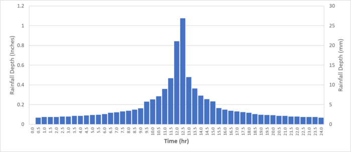
The following grid resolutions were used to test the impact of cell size on the assessment results and simulation time:
- 10ft (3.0m) cell resolution – 5,821,533 total cell count
- 12ft (3.7m) cell resolution – 4,042,960 total cell count
- 15ft (4.6m) cell resolution – 2,587,629 total cell count
- 20ft (6.1m) cell resolution – 1,455,869 total cell count
- 30ft (9.1m) cell resolution – 647,003 total cell count
- 50ft (15.2m) cell resolution – 232,957 total cell count
- 75ft (22.9m) cell resolution – 103,525 total cell count
Since the direct rainfall modelling approach means the entire model is "wet", output has been filtered to only show results in locations where the flood depth exceeds 0.3ft. This is done in TUFLOW using the TCF command "Map Cutoff Depth == ".
Test Case 2 - Results
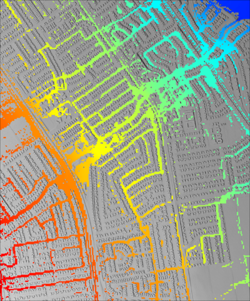
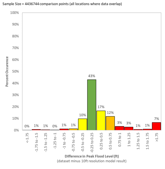
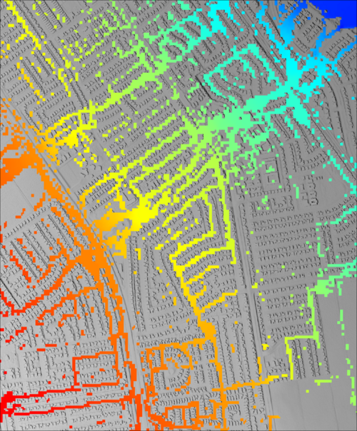
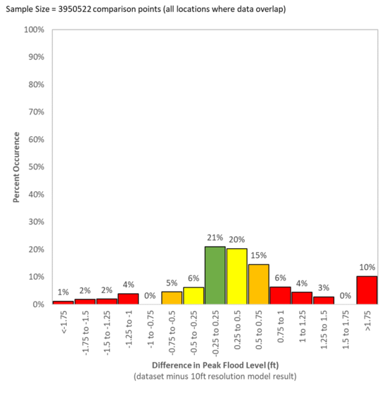
The cell convergence test results are summarised in the table below. They have been presented in a histogram form. The histograms are calculated by subtracting the peak (maximum) flood level result raster grid for the larger cell resolution simulation from the 10ft cell resolution result. The result difference has been sampled at every pixel in the raster datasets where flood information is present in both result files (i.e. they overlap).
Test Case 2 - Discussion
The urban model testing indicates result convergence occurs when the cell resolution is less than 20ft. This observation agrees with the ARR guideline recommendation for urban models to use a cell resolution of
2m (6.6ft) to 5m (16.4ft).
| Cell Size | Model Size (Cell Count) |
Simulation Run Time (hours) |
Judgement of Convergence (Yes / No) |
Required GPU Memory (GB) |
| 10ft (3.0m) | 5,821,533 | 9.2hr | Yes | 1.74 |
| 12ft (3.7m) | 4,042,960 | 7.5hr | Yes | 1.20 |
| 15ft (4.6m) | 2,587,629 | 4.4hr | Yes | 0.77 |
| 20ft (6.1m) | 1,455,869 | 1.8hr | Yes | 0.44 |
| 30ft (9.1m) | 647,003 | 0.65hr | Mostly | 0.20 |
| 50ft (15.2m) | 232,957 | 0.23hr | No | 0.07 |
| 75ft (22.9m) | 103,525 | 0.08hr | No | 0.03 |
As per Test Case 1, selection of the appropriate cell resolution during a real-world project requires consideration of the intended use of the results and also how the simulation run time impacts the overall project timeline.
- Detailed integrated 1D/2D urban modelling may adopt the 15ft (4.6m) or slightly finer 12ft (3.7m) cell resolution if the cumulative simulation time for all model events/scenarios does not adversely impact the project timeline. This timeframe consideration is particularly relevant in locations such as Australia where an ensemble methodology is currently replacing single event approaches as a way to address uncertainty associated with hydrologic assumptions.
- Broad-scale quick run simulation for urban flood forecasting purposes may adopt a coarser 20ft cell resolution or investigate the suitability of a 25ft cell resolution to achieve a quicker simulation turnaround time.
Common Questions Answered (FAQ)
How much will my runtime change when changing cell size?
Solution time for a model is dependent on a number of factors: the solution scheme used, the size and duration of the model, the nature of the hydraulics within the model, the model features selected, and the hardware that it is executed on. However, once a model is developed at a relatively coarse resolution, there are some guidelines that can assist with predicting what the solve time will be as the resolution is refined. These can be useful for estimating whether the refined model will run overnight or need a few days.
TUFLOW classic uses an implicit solution scheme that sweeps along columns and rows of cells. The solution scheme is one of the most efficient ever devised for solving the Shallow Water Equations (SWEs), but cannot be parallelised as the order of calculations are not independent. As a result the code is written to execute on a single core of a CPU. The time required to solve a model is almost exactly proportional to the number of wet cells in the model and the number of timesteps required. When the model cell size is halved, the number of cells increases by a factor of 4, and the timestep reduces by a factor of 2, so the model solve time increases by very close to a factor of 8.
TUFLOW HPC uses an explicit solution scheme, for which the cell-based calculations are able to be performed in parallel. This can be done using multiple cores of the CPU, but it is more efficiently done using the many thousands of cores of modern GPUs. The model is cut into small tiles that are divided up amongst the streaming multi-controllers (SMs) of the GPU, with each SM distributing the cell calculations of its tile amongst its cores. However, there are still some calculations that must be done at the ‘top-level’ of the model, such as updating boundary flows and levels, extracting the plot output data, timestep control, and the process of configuring and launching the GPU parallel code. These tasks remain on the CPU and cannot be parallelised as the order of execution of these instructions is vitally important. So the overall model execution contains a mix of both parallel and serial work, with the total model solve time being the sum of both. As a result, the solve time for a model doesn’t follow a simple scaling rule. The cell-based component is still proportional to the number of cells times the number of timesteps, whereas the serial component of the work is generally only proportional to the number of timesteps. To be correct, this was also true of the single core solver for TUFLOW classic, but because the cell-based component was generally more than 99% of the work load, the scaling followed the simple rule of 8 times longer for half the cell size.
In summary, for small models running with TUFLOW HPC, the solution time will increase by a factor somewhere in the range of 3 to 8 for a halving of the cell size. Once the model is sufficiently large that the cell-based calculations (running in parallel on the GPU) are taking most of the time, the time increase factor becomes close to 8. Exactly what is a “large” model will depend of the relative speed of the GPU and CPU. For that latest GPUS (as of 2021 this means the Nvidia A100 and RTX 30xx series) large typically means well over a million cells.
However, there is one last and important caveat when refining cell size. The explicit algorithm used by TUFLOW HPC requires that the timestep is also subject to Peclet (diffusion) number control, not just Courant (velocity) number control. As Peclet number is inversely proportional to cell size squared, whereas Courant number is just inversely proportional to cell size, the model will transition from Courant number control to Peclet number control once the cell size becomes small enough. This means that the factor of 8 on time for a halving of cell size will eventually become a factor of 16. This was not a feature of TUFLOW Classic. In general, we do not recommend refining cell size well into the region where timestep control is completely dominated by the Peclet number (the Nd column in the HPC output). The flows in the primary channels are usually well converged by this point, and the 2D map outputs may not reveal a lot of additional detail in the velocity fields.
| Up |
|---|
