Manhole Simple Loss Example: Difference between revisions
Tuflowduncan (talk | contribs) |
No edit summary |
||
| (32 intermediate revisions by one other user not shown) | |||
| Line 57: | Line 57: | ||
<br> |
<br> |
||
Entry losses are applied as an exit loss on the incoming conduit and are calculated as follows:<br> |
Entry losses are applied as an exit loss on the incoming conduit and are calculated as follows:<br> |
||
{{math>{K}_{\mathit{entry}}={\left\lbrack 1-\mathit{\min }\left(\frac{{V}_{m}}{{V}_{p}},1\right)\right\rbrack }^{2}</math}} |
|||
[[File:K entry.PNG]] |
[[File:K entry.PNG]] |
||
<br> |
<br> |
||
Where: |
Where:<br> |
||
[[File:Vp.PNG]] |
[[File:Vp.PNG]] |
||
<br> |
<br> |
||
With other parameters defined in the section above. The calculated flow area in the manhole is 3.6m<sup>2</sup> and 1m<sup>2</sup> in the adjacent culvert whilst the flow is 2m<sup>3</sup>/s for both Q<sub>p</sub> and Q<sub>om</sub>. |
With other parameters defined in the section above. The calculated flow area in the manhole is 3.6m<sup>2</sup> and 1m<sup>2</sup> in the adjacent culvert whilst the flow is 2m<sup>3</sup>/s for both Q<sub>p</sub> and Q<sub>om</sub>. |
||
Therefore, V<sub>m</sub> equals: |
Therefore, V<sub>m</sub> equals:<br> |
||
[[File:Vm1.PNG]] |
[[File:Vm1.PNG]]<br> |
||
And V<sub>p</sub>: |
And V<sub>p</sub>:<br> |
||
[[File:VP1.PNG]] |
[[File:VP1.PNG]] |
||
<br> |
<br> |
||
Using these in the K<sub>entry</sub> equation provides a loss coefficient of: |
Using these in the K<sub>entry</sub> equation provides a loss coefficient of:<br> |
||
[[File:K entry1.PNG]] |
[[File:K entry1.PNG]] |
||
<br> |
<br> |
||
| Line 77: | Line 74: | ||
===Example 1 - Exit Losses=== |
===Example 1 - Exit Losses=== |
||
Exit losses are applied to the upstream end of the outgoing conduit and are calculated as follows: [[File:K exit.PNG]] |
Exit losses are applied to the upstream end of the outgoing conduit and are calculated as follows:<br> [[File:K exit.PNG]]<br> |
||
<br> |
|||
| ⚫ | |||
<br> |
<br> |
||
| ⚫ | |||
Figure 3 shows that the calculated value matches those provided in the TUFLOW results. The value is also reported as the first value for the downstream conduit in the *_TSL_P.shp layer. |
Figure 3 shows that the calculated value matches those provided in the TUFLOW results. The value is also reported as the first value for the downstream conduit in the *_TSL_P.shp layer. |
||
===Example 1 - Outgoing Conduit Losses=== |
===Example 1 - Outgoing Conduit Losses=== |
||
The loss coefficient for the outgoing pipe represents the losses due to the incoming angle of the upstream conduit, any drops in inverts levels between the incoming and outgoing conduits, bend losses and any additional form losses. It is calculated as follows: |
The loss coefficient for the outgoing pipe represents the losses due to the incoming angle of the upstream conduit, any drops in inverts levels between the incoming and outgoing conduits, bend losses and any additional form losses. It is calculated as follows:<br> |
||
[[File:K outletpipe.PNG]] |
[[File:K outletpipe.PNG]]<Br> |
||
The default value of K<sub>Bend_max</sub> is set to 4 but can be changed via the 1d_mh K_Bend_Max attribute. As shown above we have no angle for the incoming pipe and no drop in invert levels. Table 1 shows the K_Fixed is equal to 2 and the outgoing pipe has a form loss coefficient, to represent bend losses of 1. Therefore K<sub>outletpipe</sub> is: |
The default value of K<sub>Bend_max</sub> is set to 4 but can be changed via the 1d_mh K_Bend_Max attribute. As shown above we have no angle for the incoming pipe and no drop in invert levels. Table 1 shows the K_Fixed is equal to 2 and the outgoing pipe has a form loss coefficient, to represent bend losses of 1. Therefore K<sub>outletpipe</sub> is:<br> |
||
[[File:K outletpipe1.PNG]] |
[[File:K outletpipe1.PNG]] |
||
| Line 134: | Line 131: | ||
In this example, the flow area in the manhole is 4.12m<sup>2</sup> and 1m<sup>2</sup> in the adjacent culvert whilst the flow is 2m<sup>3</sup>/s for both Q<sub>p</sub> and Q<sub>om</sub>. |
In this example, the flow area in the manhole is 4.12m<sup>2</sup> and 1m<sup>2</sup> in the adjacent culvert whilst the flow is 2m<sup>3</sup>/s for both Q<sub>p</sub> and Q<sub>om</sub>. |
||
Therefore, Vm equals: |
Therefore, Vm equals:<br> |
||
[[File:Vm2.PNG]] |
[[File:Vm2.PNG]] |
||
<br> |
<br> |
||
And V<sub>p</sub>: |
And V<sub>p</sub>:<br> |
||
[[File:Vp2.PNG]] |
[[File:Vp2.PNG]] |
||
<br> |
<br> |
||
From this: |
From this:<br> |
||
[[File:K entry2.PNG]] |
[[File:K entry2.PNG]] |
||
| Line 147: | Line 144: | ||
===Example 2 - Exit Losses=== |
===Example 2 - Exit Losses=== |
||
In this example, A'<sub>m</sub> is 4.12m<sup>2</sup>, therefore K<sub>exit</sub>:[[File:K exit2.PNG]] |
In this example, A'<sub>m</sub> is 4.12m<sup>2</sup>, therefore K<sub>exit</sub>:<br>[[File:K exit2.PNG]]<br> |
||
Which matches the result in figure 6. |
Which matches the result in figure 6. |
||
===Example 2 - Outgoing Conduit Losses=== |
===Example 2 - Outgoing Conduit Losses=== |
||
On this occasion, we have an 90 degree angle between the incoming and outgoing conduit. Therefore, we need to calculate Kθ using the following equation: [[File:Ktheta.PNG]] |
On this occasion, we have an 90 degree angle between the incoming and outgoing conduit. Therefore, we need to calculate Kθ using the following equation:<br> [[File:Ktheta.PNG]]<br> |
||
<br> |
<br> |
||
Q<sub>f</sub> is calculated as: [[File:Qf.PNG]] |
Q<sub>f</sub> is calculated as:<br> [[File:Qf.PNG]] |
||
<br> |
<br> |
||
Q<sub>p</sub> and Q<sub>om</sub> are both 2m<sup>3</sup>s<sup>-1</sup> and therefore Q<sub>f</sub> is equal to 1. The incoming conduit angle is 90 degrees which is cancelled out by the denominator. K<sub>θ</sub> is therefore:[[File:Ktheta1.PNG]] |
Q<sub>p</sub> and Q<sub>om</sub> are both 2m<sup>3</sup>s<sup>-1</sup> and therefore Q<sub>f</sub> is equal to 1. The incoming conduit angle is 90 degrees which is cancelled out by the denominator. K<sub>θ</sub> is therefore:<br>[[File:Ktheta1.PNG]]<br> |
||
We also have a drop between the incoming and outgoing pipes. K<sub>drop</sub> which represents losses due to this drop is calculated as follows:[[File:Kdrop.PNG]] |
We also have a drop between the incoming and outgoing pipes. K<sub>drop</sub> which represents losses due to this drop is calculated as follows:<br>[[File:Kdrop.PNG]]<br> |
||
Which is:[[File:Kdrop 1.PNG]] |
Which is:<br>[[File:Kdrop 1.PNG]]<br> |
||
Therefore K<sub>outletpipe</sub> is:[[File:K outletpipe2.PNG]] |
Therefore K<sub>outletpipe</sub> is:<br>[[File:K outletpipe2.PNG]]<br> |
||
This matches the simulated value in figure 6. |
This matches the simulated value in figure 6. |
||
| Line 168: | Line 165: | ||
==Example 3: Multiple Incoming Conduits with Incoming Bend and Drop in Invert Levels== |
==Example 3: Multiple Incoming Conduits with Incoming Bend and Drop in Invert Levels== |
||
In this example we have multiple incoming conduit. Each upstream conduit has a flow of 1m<sup>3</sup>s<sup>-1</sup> applied to it. |
In this example we have multiple incoming conduit. Each upstream conduit has a flow of 1m<sup>3</sup>s<sup>-1</sup> applied to it.<br> |
||
[[File:Schematic 3.png|800px]] |
[[File:Schematic 3.png|800px]] |
||
| Line 187: | Line 184: | ||
|'''Downstream Invert Level (m AD)''' || 99.7 || 99.8 |
|'''Downstream Invert Level (m AD)''' || 99.7 || 99.8 |
||
|} |
|} |
||
<br> |
|||
The resulting simulated loss values are presented in Figure 8. |
The resulting simulated loss values are presented in Figure 8. |
||
<br> |
<br> |
||
| Line 195: | Line 192: | ||
<br> |
<br> |
||
===Example 3 - Entry Losses=== |
===Example 3 - Entry Losses=== |
||
| ⚫ | |||
<br> |
<br> |
||
| ⚫ | |||
| ⚫ | |||
<br> |
<br> |
||
| ⚫ | |||
| ⚫ | |||
<br> |
|||
| ⚫ | |||
| ⚫ | |||
| ⚫ | |||
This matches the losses for both incoming pipes as shown in figure 8. |
This matches the losses for both incoming pipes as shown in figure 8. |
||
===Example 3 - Exit Losses=== |
===Example 3 - Exit Losses=== |
||
A'<sub>m</sub> is 3.57m<sup>2</sup> respectively. Therefore, K<sup>exit</sup>:[[File:K exit3.PNG]] |
A'<sub>m</sub> is 3.57m<sup>2</sup> respectively. Therefore, K<sup>exit</sup>:<br>[[File:K exit3.PNG]]<br> |
||
The calculated losses match the losses calculated by the TUFLOW presented in Figure 8. |
The calculated losses match the losses calculated by the TUFLOW presented in Figure 8.<br> |
||
===Example 3 - Outgoing Conduit Losses=== |
===Example 3 - Outgoing Conduit Losses===<br> |
||
In this model we have two incoming pipes, one with an 90 degree angle between the incoming and outgoing conduit and one with zero. |
In this model we have two incoming pipes, one with an 90 degree angle between the incoming and outgoing conduit and one with zero. |
||
Recall that: [[File:Ktheta.PNG]] |
Recall that: <br>[[File:Ktheta.PNG]]<br> |
||
With Qf calculated as: [[File:Qf.PNG]] |
With Qf calculated as: <br>[[File:Qf.PNG]] |
||
<br> |
<br> |
||
Q<sub>p</sub> is set to 1m<sup>3</sup>s<sup>-1</sup> and Q<sub>om</sub> to 2m<sup>3</sup>s<sup>-1</sup>. Q<sub>f</sub> is equal to 0.5m<sup>3</sup>s<sup>-1</sup>. For the incoming conduit with an angle of 90 degrees, K<sub>θ</sub> is therefore: [[File:Ktheta2a.PNG]] |
Q<sub>p</sub> is set to 1m<sup>3</sup>s<sup>-1</sup> and Q<sub>om</sub> to 2m<sup>3</sup>s<sup>-1</sup>. Q<sub>f</sub> is equal to 0.5m<sup>3</sup>s<sup>-1</sup>. For the incoming conduit with an angle of 90 degrees, K<sub>θ</sub> is therefore: <br>[[File:Ktheta2a.PNG]]<br> |
||
For the incoming conduit with an angle of 0 degrees, K<sub>θ</sub> is therefore: [[File:Ktheta2b.PNG]] |
For the incoming conduit with an angle of 0 degrees, K<sub>θ</sub> is therefore: <br>[[File:Ktheta2b.PNG]]<br> |
||
We also have a drop between the incoming and outgoing pipes. K<sub>drop</sub> which represents losses due to this drop is calculated as follows: [[File:Kdrop 2a.PNG]] |
We also have a drop between the incoming and outgoing pipes. K<sub>drop</sub> which represents losses due to this drop is calculated as follows: <br>[[File:Kdrop 2a.PNG]] |
||
<br> |
<br> |
||
and:[[File:Kdrop 2b.PNG]] |
and:<br>[[File:Kdrop 2b.PNG]]<br> |
||
Therefore, K<sub>outletpipe</sub> is: [[File:K outletpipe3.PNG]] |
Therefore, K<sub>outletpipe</sub> is: <br>[[File:K outletpipe3.PNG]]<br> |
||
The calculated value matches that presented in figure 8 for the downstream conduit loss. |
The calculated value matches that presented in figure 8 for the downstream conduit loss. |
||
{{Tips Navigation |
|||
|uplink=[[1D_Manholes| Back to 1D Manholes]] |
|||
}} |
|||
Latest revision as of 11:43, 8 January 2026
Intro
The worked examples in the section below provide hand calculations of the Engelund manhole loss approach applied to three simple examples covering:
Example 1: Single Incoming/Outgoing Pipe with No Incoming Angle or Drop
A simple TUFLOW/ESTRY model was set up as shown in Figure 1 with the parameters for the manhole and the links upstream/downstream of the manhole shown in Table 1.

Figure 1: Example Model 1 Network Schematic
.
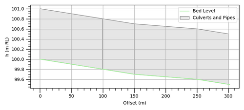
Figure 2: Example Model 1 Long Section
| Parameter | Upstream Conduit | Downstream Conduit | Manhole |
|---|---|---|---|
| ID | UC-2 | DC-1 | Manhole |
| Type | R | R | R |
| Invert Level (m AD) | N/A | N/A | 99.6 |
| Upstream Invert Level (m AD) | 99.8 | 99.7 | N/A |
| Downstream Invert Level (m AD) | 99.7 | 99.6 | N/A |
| Width(m) | 1 | N/A | 1 |
| Form Loss | 0 | 1 | N/A |
| Flow Width(m) | N/A | N/A | 1.8 |
| K_Fixed | N/A | N/A | 2 |
| Km | N/A | N/A | 1 |
Table 1: Relevant Model Parameters for Hand Calculations
The model was run with a steady inflow of 2m3s-1. The resulting losses from the 1 hour steady inflow simulation are presented in the following figure.
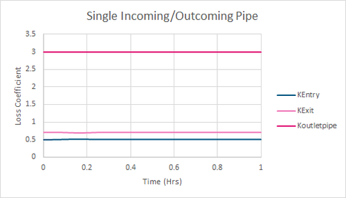
Figure 3: Example Model 1 Results-Loss Coefficients
Example 1 - Entry Losses
Entry losses are applied as an exit loss on the incoming conduit and are calculated as follows:

Where:

With other parameters defined in the section above. The calculated flow area in the manhole is 3.6m2 and 1m2 in the adjacent culvert whilst the flow is 2m3/s for both Qp and Qom.
Therefore, Vm equals:
And Vp:
Using these in the Kentry equation provides a loss coefficient of:

The value matches the downstream loss coefficient for the upstream conduit shown in Figure 3. The loss values are also shown in the *_TSL_P.shp file with the third value for the upstream conduit providing the entrance loss value.
Example 1 - Exit Losses
Exit losses are applied to the upstream end of the outgoing conduit and are calculated as follows:
From table 1, we can see that Km is set to 1. Ap and A’m are 1m2 and 3.636m2 respectively. Therefore, Kexit is:

Figure 3 shows that the calculated value matches those provided in the TUFLOW results. The value is also reported as the first value for the downstream conduit in the *_TSL_P.shp layer.
Example 1 - Outgoing Conduit Losses
The loss coefficient for the outgoing pipe represents the losses due to the incoming angle of the upstream conduit, any drops in inverts levels between the incoming and outgoing conduits, bend losses and any additional form losses. It is calculated as follows:
The default value of KBend_max is set to 4 but can be changed via the 1d_mh K_Bend_Max attribute. As shown above we have no angle for the incoming pipe and no drop in invert levels. Table 1 shows the K_Fixed is equal to 2 and the outgoing pipe has a form loss coefficient, to represent bend losses of 1. Therefore Koutletpipe is:
This matches the value within Figure 3 and the middle value for the downstream conduit in the *_TSL_P.shp, representing the outlet conduit losses, of 3.
Example 2: Single Incoming/Outgoing Conduit with Incoming Bend and Drop in Invert Levels
In this example, we will use the same simple setup but this time there is a 90 degree angle between the incoming and outgoing pipe as shown in the plan view in the figure below.
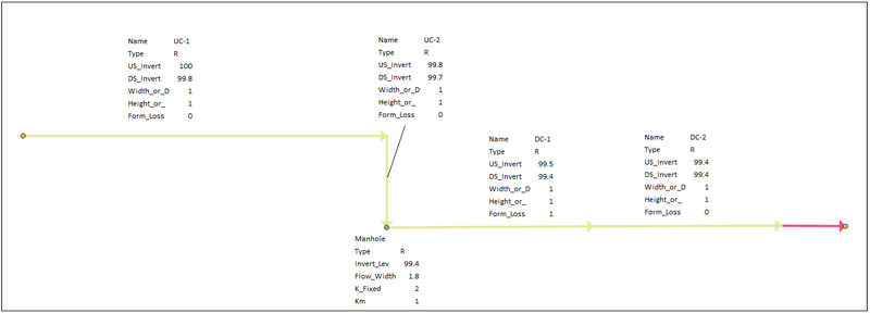
Figure 4: Example Model 2 Network Schematic
There is also a drop between the invert elevation of the incoming and outgoing conduits as shown in the difference in invert levels in table 2 below and the long profile in figure 5 . All other model parameters were kept the same including boundary inflows.
| Parameter | Upstream Conduit | Downstream Conduit | Manhole |
|---|---|---|---|
| ID | UC-2 | DC-1 | Manhole |
| Invert Level (m AD) | N/A | N/A | 99.4 |
| Upstream Invert Level (m AD) | 99.8 | 99.5 | N/A |
| Downstream Invert Level (m AD) | 99.7 | 99.4 | N/A |
Table 2: Updated Model 2 Parameters for Hand Calculations
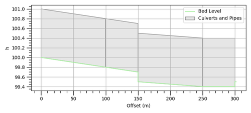
Figure 5: Example Model 2 Long Profile
The resulting simulated losses are shown in the below figure 6.
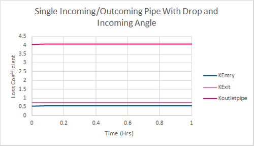
Figure 6: Example Model 2 Results-Loss Coefficients
Example 2 - Entry Losses
In this example, the flow area in the manhole is 4.12m2 and 1m2 in the adjacent culvert whilst the flow is 2m3/s for both Qp and Qom.
Therefore, Vm equals:
And Vp:
From this:

Which matches the value in figure 6.
Example 2 - Exit Losses
In this example, A'm is 4.12m2, therefore Kexit:
Which matches the result in figure 6.
Example 2 - Outgoing Conduit Losses
On this occasion, we have an 90 degree angle between the incoming and outgoing conduit. Therefore, we need to calculate Kθ using the following equation:
Qf is calculated as:

Qp and Qom are both 2m3s-1 and therefore Qf is equal to 1. The incoming conduit angle is 90 degrees which is cancelled out by the denominator. Kθ is therefore:
We also have a drop between the incoming and outgoing pipes. Kdrop which represents losses due to this drop is calculated as follows:
This matches the simulated value in figure 6.
Example 3: Multiple Incoming Conduits with Incoming Bend and Drop in Invert Levels
In this example we have multiple incoming conduit. Each upstream conduit has a flow of 1m3s-1 applied to it.
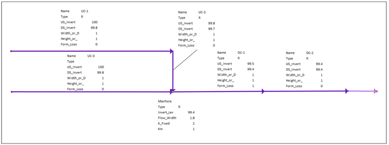
Figure 7: Example Model 3 Network Schematic
The conduits are the same shape and the same dimensions but have different invert levels as specified in the table below. All parameters for the manhole and other parts of the network are identical.
| Parameter | Upstream Conduit 1 | Upstream Conduit 2 |
|---|---|---|
| ID | UC-2 | UC-31 |
| Upstream Invert Level (m AD) | 99.8 | 100 |
| Downstream Invert Level (m AD) | 99.7 | 99.8 |
The resulting simulated loss values are presented in Figure 8.
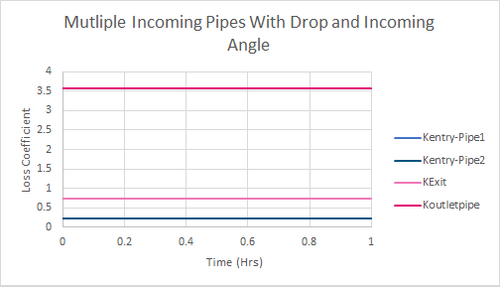
Figure 8: Example Model 3 Results-loss Coefficients
Example 3 - Entry Losses
This time the flow area in the manhole is 3.57m2 and 1m2 in the adjacent culvert whilst the flow is 1m3/s for Qp and 2m3s-1 for Qom. Therefore, Vm equals:
And Vp:
From this:
This matches the losses for both incoming pipes as shown in figure 8.
Example 3 - Exit Losses
A'm is 3.57m2 respectively. Therefore, Kexit:
The calculated losses match the losses calculated by the TUFLOW presented in Figure 8.
===Example 3 - Outgoing Conduit Losses===
In this model we have two incoming pipes, one with an 90 degree angle between the incoming and outgoing conduit and one with zero.
Recall that:
With Qf calculated as: 
Qp is set to 1m3s-1 and Qom to 2m3s-1. Qf is equal to 0.5m3s-1. For the incoming conduit with an angle of 90 degrees, Kθ is therefore:
For the incoming conduit with an angle of 0 degrees, Kθ is therefore:
We also have a drop between the incoming and outgoing pipes. Kdrop which represents losses due to this drop is calculated as follows: 
and:
The calculated value matches that presented in figure 8 for the downstream conduit loss.
| Up |
|---|


