Tutorial Module04 Archive: Difference between revisions
No edit summary |
Anne.Kolega (talk | contribs) |
||
| (11 intermediate revisions by 5 users not shown) | |||
| Line 1: | Line 1: | ||
<ol> |
<ol> |
||
=Introduction= |
=Introduction= |
||
As discussed in Module 1 [[Tutorial_Module01_Archive#Reviewing_Model_Performance | |
As discussed in Module 1 (<u>[[Tutorial_Module01_Archive#Reviewing_Model_Performance |discussion here]]</u>), the main creek channel is not very well represented using the 5m 2D cell size. In parts, the creek is only 5-10m wide and the 5m cell size could be considered too coarse to accurately represent the creek topography. Refer to the below figure.<br> |
||
[[file:Poor_2d_rep.png|400px]]<br> |
[[file:Poor_2d_rep.png|400px]]<br> |
||
Using a cell size that is coarse relative to the width of the creek channel may reduce the accuracy of the computed conveyance in the channel and introduce a source of mass error to the model. There are two options for improving the representation of the creek channel:<br> |
Using a cell size that is coarse relative to the width of the creek channel may reduce the accuracy of the computed conveyance in the channel and introduce a source of mass error to the model. There are two options for improving the representation of the creek channel:<br> |
||
* decrease the width of the 2D cells; and/or |
* decrease the width of the 2D cells; and/or |
||
* model the channel as a 1D network, dynamically linked to the 2D domain (the floodplain). |
* model the channel as a 1D network, dynamically linked to the 2D domain (the floodplain). |
||
In the optional section of module 1 [[Tutorial_Module01_Archive#Advanced_.28Optional.29 | |
In the optional section of module 1 (<u>[[Tutorial_Module01_Archive#Advanced_-_Model_Resolution_.28Optional.29 |located here]]</u>), we looked at reducing the cell size to get a better representation of the channel. In this module we will adopt the second approach of modelling the creek as 1D elements.<br> |
||
Setting up a 1D/2D model where the 1D channel cuts through the 2D domain is probably the most time-consuming type of a TUFLOW model to setup. However, the reduction in simulation time can be beneficial and make this a good approach. For this module, most of the time consuming data entry tasks have been undertaken, so you can progress through the module in a relatively short period of time. However, throughout the tutorial we will provide guidance on making this process as efficient as possible should you have to start from scratch.<br> |
Setting up a 1D/2D model where the 1D channel cuts through the 2D domain is probably the most time-consuming type of a TUFLOW model to setup. However, the reduction in simulation time can be beneficial and make this a good approach. For this module, most of the time consuming data entry tasks have been undertaken, so you can progress through the module in a relatively short period of time. However, throughout the tutorial we will provide guidance on making this process as efficient as possible should you have to start from scratch.<br> |
||
| Line 29: | Line 29: | ||
As with Modules 2 and 3 the GIS inputs are demonstrated in ArcGIS, MapInfo, SMS and QGIS. At each stage please select your GIS package for instructions. |
As with Modules 2 and 3 the GIS inputs are demonstrated in ArcGIS, MapInfo, SMS and QGIS. At each stage please select your GIS package for instructions. |
||
==1D Cross-Sections== |
==1D Cross-Sections== |
||
A 1D model requires cross-sections for processing of the channel geometry. There are a number of different formats for cross-sections to be input to TUFLOW. In this module we will be using an offset-elevation approach (XZ). This is a typical format for inputting cross-sections however, other options include height-width (HW) and MIKE11 format inputs. These are not covered in this tutorial, however the general process is very similar. To save time, the locations and XZ profiles for the 1D cross sections are provided. The XZ profiles were automatically extracted from the DEM triangulation using the 12D software (www.12d.com) with the aid of the TUFLOW utility |
A 1D model requires cross-sections for processing of the channel geometry. There are a number of different formats for cross-sections to be input to TUFLOW. In this module we will be using an offset-elevation approach (XZ). This is a typical format for inputting cross-sections however, other options include height-width (HW) and MIKE11 format inputs. These are not covered in this tutorial, however the general process is very similar. To save time, the locations and XZ profiles for the 1D cross sections are provided. The XZ profiles were automatically extracted from the DEM triangulation using the 12D software (www.12d.com) with the aid of the TUFLOW utility 12da_to_from_GIS.exe using the -xs option (see [[12da_to_from_GIS | 12da_to_from_GIS wiki page]]). The SMS TUFLOW interface has a similar and easier process, noting that a licence for the SMS TUFLOW interface is required to save the cross-sections. It is more common for this information to come from surveyed cross-sections. If the survey has been provided as x-y-z points, or a a GIS layer of points, the xs_Generator utility can be used to create the cross-sections in a TUFLOW format. The xs_Generator utility is described in the [[XsGenerator |XsGenerator wiki page]].<br> |
||
<br> |
<br> |
||
For each cross-section there is an individual comma separated variable (.csv) file. The 1d_xs layer contains a link to the source .csv file at every cross-section location. <br> |
For each cross-section there is an individual comma separated variable (.csv) file. The 1d_xs layer contains a link to the source .csv file at every cross-section location. <br> |
||
| Line 50: | Line 50: | ||
==1D Channels== |
==1D Channels== |
||
Now that we have looked at the cross section data, we must add 1D channels for the 1D network. In TUFLOW, cross sections can either be located at the ends of each channel reach, or at some point along the reach. The way that TUFLOW uses the cross-section depends upon the location, for example a "centre" cross-section has a higher priority than "end" sections if both "End" and "Centre" sections are defined. For more information on the 1D topography, |
Now that we have looked at the cross section data, we must add 1D channels for the 1D network. In TUFLOW, cross sections can either be located at the ends of each channel reach, or at some point along the reach. The way that TUFLOW uses the cross-section depends upon the location, for example a "centre" cross-section has a higher priority than "end" sections if both "End" and "Centre" sections are defined. For more information on the 1D topography, please refer to the <u>[https://docs.tuflow.com/classic-hpc/manual/latest/ TUFLOW Manual]</u>.<br> |
||
<br> |
<br> |
||
For this tutorial, we will locate most of the cross-sections at the ends of channels. There are a number of locations where a "centre" section will be used. The final channel will be a weir type channel; this represents a weir with a known stage-discharge curve. In later modules we will also use "centre" cross sections for the modelling of structures.<br> |
For this tutorial, we will locate most of the cross-sections at the ends of channels. There are a number of locations where a "centre" section will be used. The final channel will be a weir type channel; this represents a weir with a known stage-discharge curve. In later modules we will also use "centre" cross sections for the modelling of structures.<br> |
||
| Line 63: | Line 63: | ||
==1D/2D Links== |
==1D/2D Links== |
||
In this section we define lines where there is flow exchange between the 1D and 2D components of the model. At first it may seem slightly complicated, but it is actually very logical and the method allows the user to change the 2D cell size and orientation at a later stage without having to change the 1D/2D linking. Before we begin creating the link we will spend a bit of time describing how the link works. More details on the 1D/2D link can be found in |
In this section we define lines where there is flow exchange between the 1D and 2D components of the model. At first it may seem slightly complicated, but it is actually very logical and the method allows the user to change the 2D cell size and orientation at a later stage without having to change the 1D/2D linking. Before we begin creating the link we will spend a bit of time describing how the link works. More details on the 1D/2D link can be found in the <u>[https://docs.tuflow.com/classic-hpc/manual/latest/ TUFLOW Manual]</u>.<br> |
||
<br> |
<br> |
||
'''Description of linking concept'''<br> |
'''Description of linking concept'''<br> |
||
| Line 90: | Line 90: | ||
==2D Breaklines== |
==2D Breaklines== |
||
As mentioned above, the water level from the 1D is transferred out to the 2D HX cells. Therefore, it is important that the 2D cell elevation reflects the level when water can spill out into the 2D. The water level computation point for the 2D cells is the cell centre, therefore it is important to use a "thick" breakline. The types of breaklines was discussed further when reviewing the check files for the previous module <u>[[ |
As mentioned above, the water level from the 1D is transferred out to the 2D HX cells. Therefore, it is important that the 2D cell elevation reflects the level when water can spill out into the 2D. The water level computation point for the 2D cells is the cell centre, therefore it is important to use a "thick" breakline. The types of breaklines was discussed further when reviewing the check files for the previous module <u>[[Tutorial_Module03_Archive#Review_Check_Files | here]]</u>.<br> |
||
In the image below, the lightly shaded cells are the 1D/2D boundary cells. The black labels are the elevations with no breakline (elevation as read from the DEM). At the circled cell, the cell centre elevation is 44.35, this controls when water can spill from the 1D to the 2D. The red line indicates the true top of bank; the labels are elevations along this line. If this is included as a breakline, the elevations are as labelled in yellow. In this case, the level at the circled cell is actually 44.57. Including breaklines for the top of bank is important, particularly if there is an embankment or levee. |
In the image below, the lightly shaded cells are the 1D/2D boundary cells. The black labels are the elevations with no breakline (elevation as read from the DEM). At the circled cell, the cell centre elevation is 44.35, this controls when water can spill from the 1D to the 2D. The red line indicates the true top of bank; the labels are elevations along this line. If this is included as a breakline, the elevations are as labelled in yellow. In this case, the level at the circled cell is actually 44.57. Including breaklines for the top of bank is important, particularly if there is an embankment or levee. |
||
<br> |
<br> |
||
| Line 149: | Line 149: | ||
<li>After this command in the .tcf, add the following command to link the new 1D control file:</li> |
<li>After this command in the .tcf, add the following command to link the new 1D control file:</li> |
||
<font color="blue"><tt>ESTRY Control File </tt></font> <font color="red"><tt>== </tt></font> <tt>..\model\M04_1d_001.ecf</tt><br> |
<font color="blue"><tt>ESTRY Control File </tt></font> <font color="red"><tt>== </tt></font> <tt>..\model\M04_1d_001.ecf</tt><br> |
||
<li>Depending on the speed of your computer, you may have noticed in the previous three modules that when TUFLOW is running, it is hard to read the TUFLOW console output because it updates too quickly. We can reduce the frequency of output to the |
<li>Depending on the speed of your computer, you may have noticed in the previous three modules that when TUFLOW is running, it is hard to read the TUFLOW console output because it updates too quickly. We can reduce the frequency of output to the console window and also the TUFLOW Log File (.tlf). Include the following command at the end of the .tcf with the other output commands:<br> |
||
<font color="blue"><tt>Screen/Log Display Interval </tt></font> <font color="red"><tt>== </tt></font> <tt>40</tt><br> |
<font color="blue"><tt>Screen/Log Display Interval </tt></font> <font color="red"><tt>== </tt></font> <tt>40</tt><br> |
||
TUFLOW will write the output every 40 timesteps. For the 1.5 second timestep this means we will get output every 60 seconds of simulation time.<br> |
TUFLOW will write the output every 40 timesteps. For the 1.5 second timestep this means we will get output every 60 seconds of simulation time.<br> |
||
| Line 157: | Line 157: | ||
'''SMS''' users do not need to modify the control files manually because the control cards/files are automatically generated by SMS while exporting TUFLOW files. Follow ''[[Tute_M04_SMS_Simulation_Setup_Archive|these steps to Setup the Simulation]]''.<br> |
'''SMS''' users do not need to modify the control files manually because the control cards/files are automatically generated by SMS while exporting TUFLOW files. Follow ''[[Tute_M04_SMS_Simulation_Setup_Archive|these steps to Setup the Simulation]]''.<br> |
||
For all other model development platforms ( |
For all other model development platforms (e.g. ArcGIS, QGIS, MapInfo etc.)<br> |
||
<ol> |
<ol> |
||
<li>Navigate to the '''M04_1d_001.ecf''' tab or open this file.</li> |
<li>Navigate to the '''M04_1d_001.ecf''' tab or open this file.</li> |
||
| Line 232: | Line 232: | ||
==Boundary Database (bc_dbase)== |
==Boundary Database (bc_dbase)== |
||
The revised boundary data has been provided for this tutorial. This includes the stage-discharge boundary for the weir at the downstream end of the model. <br> |
The revised boundary data has been provided for this tutorial. This includes the stage-discharge boundary for the weir at the downstream end of the model. <br> |
||
Copy the '''bc_dbase_M04.csv''' and '''Weir_HQ.csv''' for the '''Module_Data\Module_4''' into the '''TUFLOW\bc_dbase\''' folder. |
Copy the '''bc_dbase_M04.csv''' and '''Weir_HQ.csv''' for the '''Module_Data\Module_4''' into the '''TUFLOW\bc_dbase\''' folder. |
||
=Run the Simulation= |
=Run the Simulation= |
||
Using your preferred method for starting TUFLOW, run the recently created '''M04_5m_001.tcf'''. Please refer to [[Tutorial_Module01_Archive# |
Using your preferred method for starting TUFLOW, run the recently created '''M04_5m_001.tcf'''. Please refer to <u>[[Tutorial_Module01_Archive#Run_Simulation | Module 1]]</u> for a detailed description of the various methods for running a TUFLOW simulation.<br> |
||
If the model fails to start correctly please refer to the <u>[[Tutorial_Module04_Archive#Troubleshooting |troubleshooting section]]</u> at the end of this page.<br> |
If the model fails to start correctly please refer to the <u>[[Tutorial_Module04_Archive#Troubleshooting |troubleshooting section]]</u> at the end of this page.<br> |
||
| Line 258: | Line 258: | ||
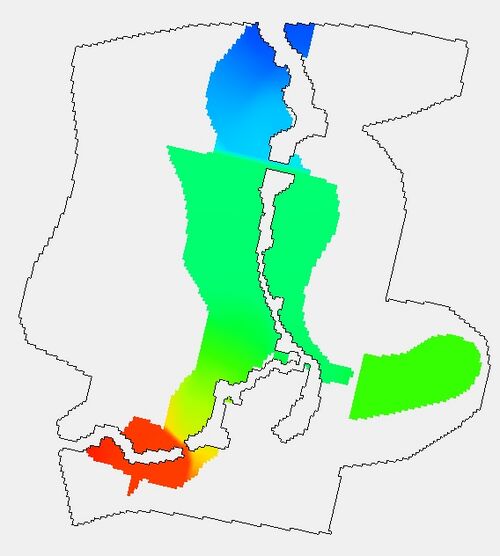
[[File:Tute M04 results no 1d 02.jpg|500px]] |
[[File:Tute M04 results no 1d 02.jpg|500px]] |
||
<br><br> |
<br><br> |
||
If you look at the 1D results (by importing the time series (_TS.mif or _TS_P.shp from the 1D results folder, or opening the M04_5m_001_1d_Q.csv) the 1D channels are conveying flow. In order to get map output for the 1D we need to use Water Level Line (WLL) inputs. The underlying water level from the 1D model is displayed across this line and as such it should be digitised perpendicular to flow. The theory behind water level lines and their use is detailed in the |
If you look at the 1D results (by importing the time series (_TS.mif or _TS_P.shp from the 1D results folder, or opening the M04_5m_001_1d_Q.csv) the 1D channels are conveying flow. In order to get map output for the 1D we need to use Water Level Line (WLL) inputs. The underlying water level from the 1D model is displayed across this line and as such it should be digitised perpendicular to flow. The theory behind water level lines and their use is detailed in the <u>[https://docs.tuflow.com/classic-hpc/manual/latest/ TUFLOW Manual]</u>. <br> |
||
<li> For the purpose of this tutorial the 1D_WLL GIS inputs have been provided for you.<br> |
<li> For the purpose of this tutorial the 1D_WLL GIS inputs have been provided for you.<br> |
||
| Line 281: | Line 281: | ||
If the TUFLOW simulation fails to start TUFLOW will output the error in a number of locations. Firstly, check the Console Window or the TUFLOW Log File (.tlf) (located in the '''TUFLOW\runs\log\''' folder with the name '''M04_5m_001.tlf'''). This file can be opened in a text editor and the error is generally located at the end of the file. You can however search for "Error" if you can not see the error. In most cases there is also a spatial location for the error message (if the error reported in the log file is prefixed by XY:). To check the location of the geographic errors, open the '''M04_5m_001_messages.mif''' or '''M04_5m_001_messages_P.shp''' file in your GIS package.<br> |
If the TUFLOW simulation fails to start TUFLOW will output the error in a number of locations. Firstly, check the Console Window or the TUFLOW Log File (.tlf) (located in the '''TUFLOW\runs\log\''' folder with the name '''M04_5m_001.tlf'''). This file can be opened in a text editor and the error is generally located at the end of the file. You can however search for "Error" if you can not see the error. In most cases there is also a spatial location for the error message (if the error reported in the log file is prefixed by XY:). To check the location of the geographic errors, open the '''M04_5m_001_messages.mif''' or '''M04_5m_001_messages_P.shp''' file in your GIS package.<br> |
||
<br> |
<br> |
||
This section contains links to some possible problems that may occur when progressing through the fourth tutorial module. If you experience an issue that is not detailed, please email support@tuflow.com |
This section contains links to some possible problems that may occur when progressing through the fourth tutorial module. If you experience an issue that is not detailed, please email [mailto:support@tuflow.com support@tuflow.com].<br> |
||
*[[Save_Date_Error_Archive|Save date of .tab file is later than .mif or .mid]] |
*[[Save_Date_Error_Archive|Save date of .tab file is later than .mif or .mid]] |
||
*[[Model_Changes_Not_Seen_Archive | When reviewing check files, I can't see the changes]] |
*[[Model_Changes_Not_Seen_Archive | When reviewing check files, I can't see the changes]] |
||
*[[Tute_Error_2051_Archive | Error 2051 - Connection object unused]] |
*[[Tute_Error_2051_Archive | Error 2051 - Connection object unused]] |
||
*[[ |
*[[TUFLOW_Message_2060 | Error 2060 - Could not find a CN connection snapped to the end of HX line]] |
||
*[[ |
*[[TUFLOW_Message_2024 | Error 2024 - Could not find a 1D node snapped to CN line.]] |
||
*[[ |
*[[Only_TUFLOW_Console_Window_Archive | Why does the TUFLOW console window open, though the TCF isn’t read and the simulation doesn’t execute?]] |
||
= Advanced - HPC Solver (Optional) = |
= Advanced - HPC Solver (Optional) = |
||
This section will introduce how to run the model TUFLOW’s HPC (Heavily Parallelised Compute) solver, and how to fix some common issues that may occur when trying to run a simulation using Graphics Processing Unit (GPU) hardware. |
This section will introduce how to run the model TUFLOW’s HPC (Heavily Parallelised Compute) solver, and how to fix some common issues that may occur when trying to run a simulation using Graphics Processing Unit (GPU) hardware. Please see [[HPC_Features_Archive | HPC Features Archive]] for more information on TUFLOW HPC features supported in the 2017 release. |
||
TUFLOW HPC can run between 10 and 100 times faster than TUFLOW Classic using NVidia Graphics Processing Units (GPU)(depending on the model configuration and hardware performance). |
TUFLOW HPC can run between 10 and 100 times faster than TUFLOW Classic using NVidia Graphics Processing Units (GPU)(depending on the model configuration and hardware performance). |
||
| Line 309: | Line 309: | ||
==Results== |
==Results== |
||
Using the methods described above in the <u>[[Tutorial_Module01_Archive#Viewing_Results | Viewing Results]]</u> section of Module 1. |
Using the methods described above in the <u>[[Tutorial_Module01_Archive#Viewing_Results | Viewing Results]]</u> section of Module 1. |
||
* Check the simulation logs in the |
* Check the simulation logs in the console window, .tlf and .hpc.tlf log files. |
||
* View the results in your preferred package. |
* View the results in your preferred package. |
||
Do the logs and results appear different to the TUFLOW Classic simulation? |
Do the logs and results appear different to the TUFLOW Classic simulation? |
||
Latest revision as of 08:21, 2 April 2026
- decrease the width of the 2D cells; and/or
- model the channel as a 1D network, dynamically linked to the 2D domain (the floodplain).
- Define 1D Cross-Sections (1d_xs)
- Define 1D Channels (1d_nwk)
- Define 1D/2D Links (2d_bc)
- Deactivate 2D Cells (2d_bc)
- Define Boundary Conditions
- Copy the Module_Data\Module_04\xs folder and all its contents to the TUFLOW\model folder (i.e. the xs folder should be located under the tuflow\model\ folder - TUFLOW\model\xs\).
- In your GIS package open the 1d_xs_M04_creek_001 file from the TUFLOW\model\xs\ folder. This is 1d_xs_M04_creek_001.tab for MapInfo users and 1d_xs_M04_creek_001_L.shp for other GIS platforms.
- Interrogate one of the cross-section lines to inspect the attributes. Notice that each line has a unique name as shown in the Source attribute, e.g. FC01 ch0834.csv. This name describes the cross section as belonging to channel FC01 at chainage 0834. The Type attribute "XZ" indicates that this cross-section is an offset-elevation type section.
- In the GIS platform a "hotlink" can be created to allow the user to open the .csv file in excel, allowing the user to easily visualise the section using an XY scatter chart type. To enable hotlinking select your GIS platform below:
- MapInfo
- ArcGIS
- QGIS
- SMS: SMS automatically extracts elevations for the HX lines when we export the TUFLOW files. Please proceed to the next section.
- Create a new 1d_bc layer and add the boundary to this; and
- Change the boundary file read into the TUFLOW boundary control file (.tbc).
- Firstly, save a copy of the TUFLOW control file created as part of Module 3 (M03_5m_001.tcf) as M04_5m_001.tcf.
- Select the lines between the start and end 1D domains (exclude the Start 1D Domain and End 1D Domain lines:
Start 1D Domain
- Output Folder == ..\results\M03\1d\
- Write Check Files == ..\check\1d\
- Output Interval (s) == 180 ! Output every 3 minutes. Note the (s) is required to output indicate value is in seconds
- Timestep == 0.75 ! Set 1D timestep to be half the 2D timestep
- Read GIS Network == ..\model\gis\1d_nwk_M02_culverts_001_L.shp
- Read GIS Network == ..\model\gis\1d_nwk_M02_culverts_001_P.shp
- Output Folder == ..\results\M03\1d\
- Copy and paste these into a new text file and save this in the TUFLOW\model\ folder as M04_1d_001.ecf. This will become our 1D control file, this will be covered in the next section.
- Delete this entire block of commands from the .tcf file (including the Start 1D Domain and End 1D Domain lines). As we have changed the geometry M03_5m_001.tgc and boundaries M02_5m_001.tbc we will need to update these files, and the links in the .tcf.
- Open the M03_5m_001.tgc and save a copy of this as M04_5m_001.tgc. Update the link in the .tcf to: Geometry Control File == ..\model\M04_5m_001.tgc
- Open the M02_5m_001.tbc and save a copy of this as M04_5m_001.tbc. Update the link in the .tcf to: BC Control File == ..\model\M04_5m_001.tbc
- We have also updated the boundary data by introducing a user specified stage-discharge relationship. The updated bc database files has been provided with the filename "bc_dbase_M04.csv". This is addressed at a later step in the model at this stage we just need to update the link in the .tcf to: BC Database == ..\bc_dbase\bc_dbase_M04.csv
- After this command in the .tcf, add the following command to link the new 1D control file: ESTRY Control File == ..\model\M04_1d_001.ecf
- Depending on the speed of your computer, you may have noticed in the previous three modules that when TUFLOW is running, it is hard to read the TUFLOW console output because it updates too quickly. We can reduce the frequency of output to the console window and also the TUFLOW Log File (.tlf). Include the following command at the end of the .tcf with the other output commands:
Screen/Log Display Interval == 40
TUFLOW will write the output every 40 timesteps. For the 1.5 second timestep this means we will get output every 60 seconds of simulation time.
This concludes the changes that we need to make to the .tcf, but before we run the model we need to update the .ecf, .tgc, .tbc and bc_dbase files. - Navigate to the M04_1d_001.ecf tab or open this file.
- Update the output folder to: Output Folder == ..\results\1D\
- We modified the culvert layer to remove the automatic 1D/2D connection.
For MapInfo Users
- The culverts (line objects) and 2D connections (point objects) are in the same GIS layer and we updated this from version 1d_nwk_M02_culverts_001 to 1d_nwk_M04_culverts_001. Update this reference in the .ecf.
- Read GIS Network == mi\1d_nwk_M04_culverts_001.mif
- We updated to the new culvert line layer, and removed the link to the points layer which contains the obsolete 1D/2D boundaries.
- To remove the culvert connections, add an exclamation mark at the start of the line, or delete the reference to 1d_nwk_M02_culverts_001_P.shp:
- Read GIS Network == gis\1d_nwk_M04_culverts_001_L.shp
- Read GIS Network == gis\1d_nwk_M02_culverts_001_P.shp
- The culverts (line objects) and 2D connections (point objects) are in the same GIS layer and we updated this from version 1d_nwk_M02_culverts_001 to 1d_nwk_M04_culverts_001. Update this reference in the .ecf.
- We also have the 1d_nwk layer for the open channel, the cross-section layer and the 1D boundary conditions. To reference these, we need to add the following lines:
For MapInfo Users
- Read GIS Network == mi\1d_nwk_M04_channels_001.mif
- Read GIS Table Links == xs\1d_xs_M04_creek_001.mif
- Read GIS BC == mi\1d_bc_M04_001.MIF
- Read GIS Network == gis\1d_nwk_M04_channels_001_L.shp
- Read GIS Table Links == xs\1d_xs_M04_creek_001_L.shp
- Read GIS BC == gis\1d_bc_M04_001_P.shp
- Read GIS Network == mi\1d_nwk_M04_channels_001.mif
- The 1D control file is now ready. Make sure you save the changes.
- We have updated the active model area;
- We have created a polygon in the 2d_bc format to deactivate the creek from the 2D model; and
- We have added a breakline to ensure the elevations of the 2D cells along the 1D/2D interface are correct.
- Open the M04_5m_001.tgc or navigate to the correct tab.
- Update the Read GIS code from 2d_code_M01_002 to 2d_code_M04_001. For MapInfo Users
- Read GIS Code == mi\2d_code_M04_001.MIF
- Read GIS Code == gis\2d_code_M04_001_R.shp
- Following the command above we need to deactivate the 2D cells in the creek. As these commands are processed in the order they are written, this must appear below the command above. Add the following command. For MapInfo, the code region is stored in the same layer as the HX lines (2d_bc_M04_HX_001) however, in ArcMap and QGIS the regions must be in a different layer than the lines and a 2d_code layer was used. Note the "BC" is required for the MapInfo input to indicate the code polygon is in a 2d_bc format and not in the 2d_code format. For MapInfo Users
- Read GIS Code BC == mi\2d_bc_M04_HX_001.mif
- Read GIS Code == gis\2d_code_M04_null_creek_001_R.shp
- To include the breakline for the top of bank add the following after the existing Read "GIS Z Shape" command. As the line and points are in separate files, we need to include both layers, these are separated by a vertical bar (|). The "MAX" option will only raise the elevation, if the existing Zpt is higher, this will not be lowered. For MapInfo Users
- Read GIS Z HX Line MAX == mi\2d_bc_M04_HX_001.mif | mi\2d_bc_M04_HX_001_P.mif
- Read GIS Z HX Line MAX == gis\2d_bc_M04_HX_001_L.shp | gis\2d_bc_M04_HX_001_P.shp
- Save the file. The geometry file is now ready to be used.
- Open M04_5m_001.tbc. The first boundary in the 2D boundary control file 2d_bc_M01_002.tbc contains the external flow boundary at the western edge of the model and the downstream HQ boundary. These boundaries have both been removed from the 2D and included in the 1D. Therefore, this layer is no longer required and leaving it would cause problems because the boundaries would be in both the 1D and the 2D. Therefore this command should be commented out or deleted. ! Read GIS BC == gis\2d_bc_M01_002_L.SHP
- In the "Internal (1D/2D) Boundaries" section of the control file we need to update the culvert boundaries to 2d_bc_M04_culverts_001. We also need to include the HX boundaries for the open channel sections. For MapInfo Users
- Read GIS BC == mi\2d_bc_M04_culverts_001.MIF
- Read GIS BC == mi\2d_bc_M04_HX_001.mif
- Comment out (or delete) the following line:
- !Read GIS BC == gis\2d_bc_M02_culv_001_L.shp
- The GIS layer 2d_bc_M02_culv_001_L.shp contains only the 1d/2d connection for the northern culvert. This culvert is now connected directly to the 1D open channel and this culvert connection is no longer required.
- Add the following line.
- Read GIS BC == gis\2d_bc_M04_HX_001_L.shp
- Save the file. The boundary file is now ready to be used.
- M04_5m_001_grd_check
- M04_5m_001_1d_to_2d_check
- M04_5m_001_zln_zpt_check
- M04_5m_001_nwk_C_check
- M03_5m_001_1d_bc_check
- Open the 2D results in your results viewer or import to your GIS package. You should see that where we have replaced the 2D with the 1D model there are no results displayed.
If you look at the 1D results (by importing the time series (_TS.mif or _TS_P.shp from the 1D results folder, or opening the M04_5m_001_1d_Q.csv) the 1D channels are conveying flow. In order to get map output for the 1D we need to use Water Level Line (WLL) inputs. The underlying water level from the 1D model is displayed across this line and as such it should be digitised perpendicular to flow. The theory behind water level lines and their use is detailed in the TUFLOW Manual.
- For the purpose of this tutorial the 1D_WLL GIS inputs have been provided for you.
For MapInfo Users
- Copy the 1d_WLL_M04_001.mif and 1d_WLLp_M04_001.mif to your TUFLOW\model\mi\ folder. Add the following to the 1D (ESTRY) control file M04_1d_001.ecf.
- Read GIS WLL == mi\1d_WLL_M04_001.mif
- Read GIS WLL Points == mi\1d_WLLp_M04_001.mif
- Copy the 1d_WLL_M04_001_L.shp and 1d_WLLp_M04_001_P.shp to your TUFLOW\model\gis\ folder. In the Estry Control File (.ecf) add the following lines:
- Read GIS WLL == gis\1d_WLL_M04_001_L.shp
- Read GIS WLL Points == gis\1d_WLLp_M04_001_P.shp
- Copy the 1d_WLL_M04_001.mif and 1d_WLLp_M04_001.mif to your TUFLOW\model\mi\ folder. Add the following to the 1D (ESTRY) control file M04_1d_001.ecf.
- Save the 1D control file and re-run the simulation. When reloaded, the 1D results should now be mapped with the 2D results as per the following image.
- Save date of .tab file is later than .mif or .mid
- When reviewing check files, I can't see the changes
- Error 2051 - Connection object unused
- Error 2060 - Could not find a CN connection snapped to the end of HX line
- Error 2024 - Could not find a 1D node snapped to CN line.
- Why does the TUFLOW console window open, though the TCF isn’t read and the simulation doesn’t execute?
- Save the TUFLOW runfile (M04_5m_001.tcf) as M04_5m_002.tcf.
- Add the following command to the TCF file:
- Solution Scheme == HPC ! Use HPC solver to run the model
- Solution Scheme == HPC ! Use HPC solver to run the model
- If you have a CUDA enabled NVIDIA GPU device, you can also add the following command to run the HPC solver using GPU hardware:
- Hardware == GPU ! Run HPC solver on GPU
- Hardware == GPU ! Run HPC solver on GPU
- Save the TCF file and run the model.
- Check the simulation logs in the console window, .tlf and .hpc.tlf log files.
- View the results in your preferred package.
- Check if your GPU card is an NVIDIA GPU card. Currently, TUFLOW does not run on AMD type GPU.
- Check if your NVIDIA GPU card is CUDA enabled and whether the latest drivers are installed. Please see GPU Setup.
Introduction
As discussed in Module 1 (discussion here), the main creek channel is not very well represented using the 5m 2D cell size. In parts, the creek is only 5-10m wide and the 5m cell size could be considered too coarse to accurately represent the creek topography. Refer to the below figure.

Using a cell size that is coarse relative to the width of the creek channel may reduce the accuracy of the computed conveyance in the channel and introduce a source of mass error to the model. There are two options for improving the representation of the creek channel:
In the optional section of module 1 (located here), we looked at reducing the cell size to get a better representation of the channel. In this module we will adopt the second approach of modelling the creek as 1D elements.
Setting up a 1D/2D model where the 1D channel cuts through the 2D domain is probably the most time-consuming type of a TUFLOW model to setup. However, the reduction in simulation time can be beneficial and make this a good approach. For this module, most of the time consuming data entry tasks have been undertaken, so you can progress through the module in a relatively short period of time. However, throughout the tutorial we will provide guidance on making this process as efficient as possible should you have to start from scratch.
There are a number of steps involved in the process.
Within our GIS platform we need to make the following changes:
We also need to modify the TUFLOW run files to reflect these new and changed GIS layers.
Model Configuration
As well as replacing the in-bank area with 1D elements, we we also extend the model further downstream. As this extends beyond the area of the DEM provided, we will transition from a 1D/2D model within the study area to a 1D only model. This allows us to extend the downstream boundary (stage-discharge boundary) further from our area of interest. We have cross-sectional details downstream of the DEM, but insufficient topography data to model this in 2D. This approach can also be used to reduce the 2D model area, thereby reducing model runtimes, or allowing a finer 2D cell size to be used.
The configuration of the model for this tutorial is provided in the image below.

Modify GIS Inputs
As with Modules 2 and 3 the GIS inputs are demonstrated in ArcGIS, MapInfo, SMS and QGIS. At each stage please select your GIS package for instructions.
1D Cross-Sections
A 1D model requires cross-sections for processing of the channel geometry. There are a number of different formats for cross-sections to be input to TUFLOW. In this module we will be using an offset-elevation approach (XZ). This is a typical format for inputting cross-sections however, other options include height-width (HW) and MIKE11 format inputs. These are not covered in this tutorial, however the general process is very similar. To save time, the locations and XZ profiles for the 1D cross sections are provided. The XZ profiles were automatically extracted from the DEM triangulation using the 12D software (www.12d.com) with the aid of the TUFLOW utility 12da_to_from_GIS.exe using the -xs option (see 12da_to_from_GIS wiki page). The SMS TUFLOW interface has a similar and easier process, noting that a licence for the SMS TUFLOW interface is required to save the cross-sections. It is more common for this information to come from surveyed cross-sections. If the survey has been provided as x-y-z points, or a a GIS layer of points, the xs_Generator utility can be used to create the cross-sections in a TUFLOW format. The xs_Generator utility is described in the XsGenerator wiki page.
For each cross-section there is an individual comma separated variable (.csv) file. The 1d_xs layer contains a link to the source .csv file at every cross-section location.
For SMS Users
For ArcGIS, MapInfo and QGIS Users
Tip: The XY scatter plot can be setup as the default chart type in excel, this makes it simple to plot the cross-sections, simply open the .csv in Excel using the GIS hotlink functionality, select the data and the hit the F11 key to create a chart. Instructions for setting an x-y scatter as the default chart type can be found in this Excel tip.
For MapInfo users with the miTools utility, the cross-sections can be viewed directly within MapInfo, instructions for doing so are in the viewing cross-sections in MapInfo with the miTools page.
Users with the SMS-TUFLOW interface can also directly view the cross-sections in the viewing cross-sections in SMS page.
1D Channels
Now that we have looked at the cross section data, we must add 1D channels for the 1D network. In TUFLOW, cross sections can either be located at the ends of each channel reach, or at some point along the reach. The way that TUFLOW uses the cross-section depends upon the location, for example a "centre" cross-section has a higher priority than "end" sections if both "End" and "Centre" sections are defined. For more information on the 1D topography, please refer to the TUFLOW Manual.
For this tutorial, we will locate most of the cross-sections at the ends of channels. There are a number of locations where a "centre" section will be used. The final channel will be a weir type channel; this represents a weir with a known stage-discharge curve. In later modules we will also use "centre" cross sections for the modelling of structures.
For the open channel type we will use three different types of channels. The three types channel types are: standard open channel (S), weir (W) and channel connector (X). The GIS "Channel_type" attribute is in brackets. The connector channel is used where there is a branch in the channel, the connector type indicates a side channel entering. This is not mandatory, but if using channel interpolation, this allows TUFLOW to determine the main channel.
As the cross sections have been provided, the digitisation of the channel is simply a matter of joining the dots. We are going to create a series of lines between the cross sections. It is important that the end of each channel snaps to a vertex along the cross-section line, so we will be using the snapping tools in the GIS. We have provided a 1d_nwk_M04_creek_001 GIS layer. This layer has the first few channels digitised for you. A revised culvert layer 1d_nwk_M04_creek_001 is also provided, this has the culverts connected to the new channels layer. The creation of the 1d network layers is described for the GIS packages below:
1D/2D Links
In this section we define lines where there is flow exchange between the 1D and 2D components of the model. At first it may seem slightly complicated, but it is actually very logical and the method allows the user to change the 2D cell size and orientation at a later stage without having to change the 1D/2D linking. Before we begin creating the link we will spend a bit of time describing how the link works. More details on the 1D/2D link can be found in the TUFLOW Manual.
Description of linking concept
We are going to apply a water level boundary to the 2D cells along the 1D/2D interface. In the 2D boundary condition (2d_bc) GIS layer, we define the location at which this link occurs. The 2D water level applied at the 2D boundary cells is calculated in the 1D model. The terminology used in TUFLOW is a "HX" type boundary on the 2D cells, with the H indicating that a Head (water level) boundary is used and the X indicating the value is coming from an eXternal model (in this case the 1D).
Using a similar naming convention, a HT boundary is a Head versus Time boundary, a QT indicates a flow-time (hydrograph) boundary and a HQ boundary used in the model is a Head versus Flow (or stage-discharge) boundary.
Depending on the water level in the surrounding 2D cells, flow can either enter or leave the "HX" cells. The volume of water entering or leaving the 2D boundary is added or subtracted from the 1D model to preserve volume. As was done in Module 2 for the SX lines, we must connect the HX lines to the 1D network. This is done using CN type lines in the 2d_bc layer, where a CN line is connected to the HX line, the water level from the 1D nodes is transferred to the HX line. In between 1D nodes a linear interpolation of water level is applied. This is shown in the image below.

As the water level in the 2D is calculated at the cell centres, once the water level in the 1D exceeds the elevation in the boundary cell water can enter or leave the model. If there is a levee, it is important that we use breaklines in the model to ensure that the elevations of the 2D cells are consistent with the levee crest. This will be described in the next section of the tutorial. The next four images show a section view of the 1D/2D link and how this may progress during a flood event.


Often HX lines are located along the top of a levee (natural or artificial) or flood defence running along the river bank. When carving a 1D channel through a 2D domain, the HX line must be either on the top of the levee or on the inside of the levee (closest to the channel). If the HX line is located on the other side of the levee away from the channel, the effect of the levee on water flow is not modelled. In the sections above, it can be seen that the boundary cell is along the levee and the interaction between the channel and the floodplain (1D and 2D) occurs at the correct elevation.
Now that we have a background in the linking approach it is time to define the 1D/2D link. This process is described for the various GIS packages in the links below:
2D Breaklines
As mentioned above, the water level from the 1D is transferred out to the 2D HX cells. Therefore, it is important that the 2D cell elevation reflects the level when water can spill out into the 2D. The water level computation point for the 2D cells is the cell centre, therefore it is important to use a "thick" breakline. The types of breaklines was discussed further when reviewing the check files for the previous module here.
In the image below, the lightly shaded cells are the 1D/2D boundary cells. The black labels are the elevations with no breakline (elevation as read from the DEM). At the circled cell, the cell centre elevation is 44.35, this controls when water can spill from the 1D to the 2D. The red line indicates the true top of bank; the labels are elevations along this line. If this is included as a breakline, the elevations are as labelled in yellow. In this case, the level at the circled cell is actually 44.57. Including breaklines for the top of bank is important, particularly if there is an embankment or levee.

To include breaklines for the top of bank, follow the instructions outlined in your GIS package below.
Deactivate 2D Cells
Now that we have defined the 1D model and the 1D/2D linking location, we need to deactivate the 2D cells where the 1D model is replacing the 2D solution. It is important that the area deactivated from the 2D is the same as the area modelled in the 1D solution. If the 1D cross sections are 20m wide, but a 40m width is removed from the 2D model, the model will be underestimating the conveyance. The opposite would be true if the 1D cross sections were 80m wide but only a 40m width had been deactivated, i.e. the model would be overestimating the conveyance.
As the HX line was created along the top of bank and was as wide as the cross-sections, we can snap the code polygon (which deactivates the 2D cells) to the HX line. To do this please select your GIS package from the list below:
Define Boundary Conditions
You may have noticed that in addition to extending downstream of the 2D active domain to the north, the 1D network extends slightly upstream from the 2D active domain at the south western edge of the model. Therefore, we need to adjust the inflow and outflow boundary locations. We are going to replace the upstream inflow boundary (QT type) which is in the 2D_bc layer, with boundaries applied at the upstream and downstream extents of the 1D network. To do this we need to:
We will be using the same boundary hydrograph and therefore will not need to update the boundary database (bc_dbase).
For the GIS changes please select your GIS package from the list below.
Modify Simulation Control Files
Now that we have made all of the necessary changes to the GIS layers, we need to update our control files to utilise the new GIS layers. Now that the 1D component of the model is becoming more complex we are going to use a separate control file for the 1D inputs. The new 1D control file will have the extension .ecf, this stands for ESTRY Control File. ESTRY was a 1D hydraulic modelling package before TUFLOW was created. The functionality of ESTRY has been incorporated in TUFLOW but for historic reasons the 1D control file is still referred to as the ESTRY Control File and has the .ecf file extension.
SMS users do not need to modify the control files manually because SMS writes out the control cards and files automatically while exporting the TUFLOW project. Please proceed to Simulation Setup.
TUFLOW Control File (TCF)
ESTRY Control File (ECF)
SMS users do not need to modify the control files manually because the control cards/files are automatically generated by SMS while exporting TUFLOW files. Follow these steps to Setup the Simulation.
For all other model development platforms (e.g. ArcGIS, QGIS, MapInfo etc.)
Note: We have removed the module number from the output folder ..\results\1D\ instead of ..\results\M04\1D\ from now on all 1D output will be written to the same folder. This is a matter of preference, TUFLOW will output the results where you want them!
TUFLOW Geometry Control (TGC) File
There have been three changes to the geometry:
TUFLOW Boundary Control (TBC) File
Boundary Database (bc_dbase)
The revised boundary data has been provided for this tutorial. This includes the stage-discharge boundary for the weir at the downstream end of the model.
Copy the bc_dbase_M04.csv and Weir_HQ.csv for the Module_Data\Module_4 into the TUFLOW\bc_dbase\ folder.
Run the Simulation
Using your preferred method for starting TUFLOW, run the recently created M04_5m_001.tcf. Please refer to Module 1 for a detailed description of the various methods for running a TUFLOW simulation.
If the model fails to start correctly please refer to the troubleshooting section at the end of this page.
Review Check Files
Once the model has started we can review the check files to ensure the changes have been correctly applied. From the TUFLOW\check\2d\ folder import (into MapInfo) or open (ArcMap and QGIS) the following check files:
From the TUFLOW\check\1d\ folder import (into MapInfo) or open (ArcMap and QGIS) the following check files:
In the creek channel we should see that there are channels in the 1D network and that the 2D grid has been deactivated. Along the HX line we should see that there are connections in the 1d_to_2d check file and that the breaklines have modified the elevations at these cells. This is shown in the image below. If these changes are not visible in your model, ensure that the correct .tcf has been run and refer to the troubleshooting section.

Review the Results


Conclusion
We have made major changes to our TUFLOW tutorial model. The open channel in now modelled in 1D, with 1D/2D connections along the top of bank. The model has also been extended further downstream (in 1D) and a user defined stage-discharge relationship has been adopted.
Congratulations on finishing Module 4!
Troubleshooting
If the TUFLOW simulation fails to start TUFLOW will output the error in a number of locations. Firstly, check the Console Window or the TUFLOW Log File (.tlf) (located in the TUFLOW\runs\log\ folder with the name M04_5m_001.tlf). This file can be opened in a text editor and the error is generally located at the end of the file. You can however search for "Error" if you can not see the error. In most cases there is also a spatial location for the error message (if the error reported in the log file is prefixed by XY:). To check the location of the geographic errors, open the M04_5m_001_messages.mif or M04_5m_001_messages_P.shp file in your GIS package.
This section contains links to some possible problems that may occur when progressing through the fourth tutorial module. If you experience an issue that is not detailed, please email support@tuflow.com.
Advanced - HPC Solver (Optional)
This section will introduce how to run the model TUFLOW’s HPC (Heavily Parallelised Compute) solver, and how to fix some common issues that may occur when trying to run a simulation using Graphics Processing Unit (GPU) hardware. Please see HPC Features Archive for more information on TUFLOW HPC features supported in the 2017 release.
TUFLOW HPC can run between 10 and 100 times faster than TUFLOW Classic using NVidia Graphics Processing Units (GPU)(depending on the model configuration and hardware performance).
Model Setup
In order to use the HPC solver, we will need to perform the following steps:
TIP: To learn how to optimise a HPC simulation to achieve the fastest simulation speed please complete Tutorial Module 2 and Tutorial Module 3
Results
Using the methods described above in the Viewing Results section of Module 1.
Do the logs and results appear different to the TUFLOW Classic simulation?
Troubleshooting for GPU Simulations
If you receive the following error when trying to run the TUFLOW HPC model using GPU hardware:
TUFLOW GPU: Interrogating CUDA enabled GPUs …
TUFLOW GPU: Error: Non-CUDA Success Code returned
or
ERROR 2785 - No GPU devices found, enabled or compatible.
Please try the following steps:
If you experience an issue that is not detailed above please send an email to support@tuflow.com