Tutorial M01: Difference between revisions
Anne.Kolega (talk | contribs) |
|||
| (24 intermediate revisions by 5 users not shown) | |||
| Line 24: | Line 24: | ||
<ol><ol><li>2d_po: A time series data output from 2D domains, for a range of hydraulic parameters. |
<ol><ol><li>2d_po: A time series data output from 2D domains, for a range of hydraulic parameters. |
||
</ol></ol> |
</ol></ol> |
||
This tutorial is setup with shapefiles (SHP) and geopackage (GPKG) layers. For more information on these formats, see <u>[https://docs.tuflow.com/classic-hpc/manual/latest/ TUFLOW Manual]</u>. |
|||
<br> |
<br> |
||
= Project Initialisation = |
= Project Initialisation = |
||
TUFLOW models are separated into a series of folders which contain the input and output files. The recommended set up for the model directory and sub-folders is shown below. For a more detailed description, |
TUFLOW models are separated into a series of folders which contain the input and output files. The recommended set up for the model directory and sub-folders is shown below. For a more detailed description, refer to the <u>[https://docs.tuflow.com/classic-hpc/manual/latest/ TUFLOW Manual]</u>. <br> |
||
<ol> |
<ol> |
||
[[File:Tute M01 Directory Structure v3.png|left]] |
[[File:Tute M01 Directory Structure v3.png|left]] |
||
| Line 46: | Line 47: | ||
| model\mi|| Input || GIS layers that are inputs to the 2D and 1D model domains are contained within this folder, model\mi is typically used for MapInfo formatted GIS files. |
| model\mi|| Input || GIS layers that are inputs to the 2D and 1D model domains are contained within this folder, model\mi is typically used for MapInfo formatted GIS files. |
||
|- |
|- |
||
| results|| Output|| TUFLOW outputs the results to this folder in |
| results|| Output|| TUFLOW outputs the results to this folder in specified formats. |
||
|- |
|- |
||
| runs|| Input|| TUFLOW Control Files (TCF). |
| runs|| Input|| TUFLOW Control Files (TCF). |
||
| Line 54: | Line 55: | ||
</ol> |
</ol> |
||
The TUFLOW folders can be set up manually, automatically running TUFLOW model with <font color="blue"><tt> Write Empty GIS Files </tt></font> command or automatically through GIS programs: |
The TUFLOW folders can be set up manually, automatically running TUFLOW model with <font color="blue"><tt> Write Empty GIS Files </tt></font> command or automatically through GIS programs: |
||
:*<u>[[Tutorial_M01_Configure_TUFLOW_Project_QGIS | QGIS]]</u> |
:*<u>[[Tutorial_M01_Configure_TUFLOW_Project_QGIS | QGIS - SHP]]</u> |
||
:*<u>[[Tutorial_M01_Configure_TUFLOW_Project_QGIS_GPKG | QGIS - GPKG]]</u> |
|||
:*SMS - the folder structure listed above is automatically created before running the model using the 'Export TUFLOW files' command (see <u> [[Run TUFLOW from within SMS | Run TUFLOW from within SMS]])</u>. |
:*SMS - the folder structure listed above is automatically created before running the model using the 'Export TUFLOW files' command (see <u> [[Run TUFLOW from within SMS | Run TUFLOW from within SMS]])</u>. |
||
:*ArcMap (10.1 and newer) - the ArcTUFLOW Toolbox can be used to automatically create the model folders, model projection, TUFLOW control files and run TUFLOW to create the template files. |
:*ArcMap (10.1 and newer) - the ArcTUFLOW Toolbox can be used to automatically create the model folders, model projection, TUFLOW control files and run TUFLOW to create the template files. |
||
| Line 80: | Line 82: | ||
=== 2D Domain === |
=== 2D Domain === |
||
Grid formats currently supported by TUFLOW include the ESRI ASCII |
Grid formats currently supported by TUFLOW include the ESRI ASCII grid format (.asc), binary grids (.flt) and geodetic grids (.tif). The Digital Elevation Model (DEM) is provided in .tif format. <br> |
||
Defining the location and orientation of the TUFLOW 2D domain can be undertaken using four different methods: <br> |
Defining the location and orientation of the TUFLOW 2D domain can be undertaken using four different methods: <br> |
||
| Line 105: | Line 107: | ||
<font color="blue"><tt>Set Code </tt></font> <font color="red"><tt>== </tt></font> <font color="black"><tt>0</tt></font> <font color="green"><tt> ! Sets all cells to inactive</tt></font> |
<font color="blue"><tt>Set Code </tt></font> <font color="red"><tt>== </tt></font> <font color="black"><tt>0</tt></font> <font color="green"><tt> ! Sets all cells to inactive</tt></font> |
||
<li>Define active areas: <br> |
<li>Define active areas: <br> |
||
:*<u>[[Tutorial_M01_Define_Active_Area_QGIS | QGIS]]</u> |
:*<u>[[Tutorial_M01_Define_Active_Area_QGIS | QGIS - SHP]]</u> |
||
:*<u>[[Tutorial_M01_Define_Active_Area_QGIS_GPKG | QGIS - GPKG]]</u> |
|||
<li>Set all cells within the code polygon to active. The command needs to be written after the <font color="blue"><tt> Set Code </tt></font> <font color="red"><tt>== </tt></font> <font color="black"><tt>0 </tt></font> command to overwrite the inactive cells within the polygon: <br> |
<li>Set all cells within the code polygon to active. The command needs to be written after the <font color="blue"><tt> Set Code </tt></font> <font color="red"><tt>== </tt></font> <font color="black"><tt>0 </tt></font> command to overwrite the inactive cells within the polygon: <br> |
||
<u>'''QGIS - SHP'''</u><br> |
|||
<font color="blue"><tt>Read GIS Code </tt></font> <font color="red"><tt>== </tt></font> <font color="black"><tt>gis\2d_code_M01_001_R.shp</tt></font> <font color="green"><tt> ! Sets cell codes according to attributes in the GIS layer</tt></font> <br> |
<font color="blue"><tt>Read GIS Code </tt></font> <font color="red"><tt>== </tt></font> <font color="black"><tt>gis\2d_code_M01_001_R.shp</tt></font> <font color="green"><tt> ! Sets cell codes according to attributes in the GIS layer</tt></font> <br> |
||
<u>'''QGIS - GPKG'''</u><br> |
|||
<font color="blue"><tt>Read GIS Code </tt></font> <font color="red"><tt>== </tt></font> <font color="black"><tt>2d_code_M01_001_R</tt></font> <font color="green"><tt> ! Sets cell codes according to attributes in the GIS layer</tt></font> <br> |
|||
</ol> |
</ol> |
||
Note: As mentioned, the order of commands in the TGC is critical. The final cell value (such as for code, elevation or material) is specified by the file lowest in the TGC. Consider the above two commands to set active and inactive cells, if the <font color="blue"><tt>Read GIS Code </tt></font> was written before the <font color="blue"><tt>Set Code </tt></font> command, all the cells within the code polygon would be first set to active and then overwritten to be all inactive, no hydraulic simulation could occur.<br> |
Note: As mentioned, the order of commands in the TGC is critical. The final cell value (such as for code, elevation or material) is specified by the file lowest in the TGC. Consider the above two commands to set active and inactive cells, if the <font color="blue"><tt>Read GIS Code </tt></font> was written before the <font color="blue"><tt>Set Code </tt></font> command, all the cells within the code polygon would be first set to active and then overwritten to be all inactive, no hydraulic simulation could occur.<br> |
||
=== Topography === |
=== Topography === |
||
The points that assign elevations at each 2D cell centre, mid-side and corner are called Zpts. For a description on the computational function of each of the Zpts in a TUFLOW cell, see <u>[https://wiki.tuflow.com/ |
The points that assign elevations at each 2D cell centre, mid-side and corner are called Zpts. For a description on the computational function of each of the Zpts in a TUFLOW cell, see <u>[https://wiki.tuflow.com/Zpt_Description Zpt Description]</u>. <br> |
||
A DEM is used to assign elevations to the Zpts: <br> |
A DEM is used to assign elevations to the Zpts: <br> |
||
<ol> |
<ol> |
||
<li>Copy the DEM ( |
<li>Copy the DEM ('''DEM.tif''') from the '''DEM''' folder into a new '''Module_01\TUFLOW\model\grid''' folder.<br> |
||
<li>Set a global elevation for the Zpts by adding the following line to the TGC file:<br> |
<li>Set a global elevation for the Zpts by adding the following line to the TGC file:<br> |
||
<font color="blue"><tt>Set Zpts </tt></font> <font color="red"><tt>== </tt></font> <font color="black"><tt> 100</tt></font> <font color="green"><tt> ! Sets every 2D elevation zpt to 100 metres</tt></font> <br> |
<font color="blue"><tt>Set Zpts </tt></font> <font color="red"><tt>== </tt></font> <font color="black"><tt> 100</tt></font> <font color="green"><tt> ! Sets every 2D elevation zpt to 100 metres</tt></font> <br> |
||
| Line 134: | Line 140: | ||
<font color="blue"><tt>Set Mat </tt></font> <font color="red"><tt>== </tt></font> <font color="black"><tt>1</tt></font> <font color="green"><tt> ! Sets all cells to a material ID of 1</tt></font><br> |
<font color="blue"><tt>Set Mat </tt></font> <font color="red"><tt>== </tt></font> <font color="black"><tt>1</tt></font> <font color="green"><tt> ! Sets all cells to a material ID of 1</tt></font><br> |
||
<li>Define spatial material definition: |
<li>Define spatial material definition: |
||
:*<u>[[Tutorial_M01_Materials_QGIS | QGIS]]</u> |
:*<u>[[Tutorial_M01_Materials_QGIS | QGIS - SHP]]</u> |
||
:*<u>[[Tutorial_M01_Materials_QGIS_GPKG | QGIS - GPKG]]</u> |
|||
<li>Assign materials from the GIS layer to overwrite the global material at all cells that fall within the material polygons: <br> |
<li>Assign materials from the GIS layer to overwrite the global material at all cells that fall within the material polygons: <br> |
||
<u>'''QGIS - SHP'''</u><br> |
|||
<font color="blue"><tt>Read GIS Mat </tt></font> <font color="red"><tt>== </tt></font> <font color="black"><tt>gis\2d_mat_M01_001_R.shp</tt></font> <font color="green"><tt> ! Sets material values according to attributes in the GIS layer</tt></font><br> |
<font color="blue"><tt>Read GIS Mat </tt></font> <font color="red"><tt>== </tt></font> <font color="black"><tt>gis\2d_mat_M01_001_R.shp</tt></font> <font color="green"><tt> ! Sets material values according to attributes in the GIS layer</tt></font><br> |
||
<u>'''QGIS - GPKG'''</u><br> |
|||
<font color="blue"><tt>Read GIS Mat </tt></font> <font color="red"><tt>== </tt></font> <font color="black"><tt>2d_mat_M01_001_R</tt></font> <font color="green"><tt> ! Sets material values according to attributes in the GIS layer</tt></font><br> |
|||
<li>Save the TGC file. |
<li>Save the TGC file. |
||
| Line 161: | Line 171: | ||
Set up boundary condition layers: <br> |
Set up boundary condition layers: <br> |
||
:*<u>[[Tutorial_M01_Boundary_Conditions_QGIS | QGIS]]</u> |
:*<u>[[Tutorial_M01_Boundary_Conditions_QGIS | QGIS - SHP]]</u> |
||
:*<u>[[Tutorial_M01_Boundary_Conditions_QGIS_GPKG | QGIS - GPKG]]</u> |
|||
=== TUFLOW Boundary Control File (TBC) === |
=== TUFLOW Boundary Control File (TBC) === |
||
| Line 168: | Line 179: | ||
<li>Create a new text file and save as '''M01_001.tbc''' in the '''Module_01\TUFLOW\model''' folder. <br> |
<li>Create a new text file and save as '''M01_001.tbc''' in the '''Module_01\TUFLOW\model''' folder. <br> |
||
<li>Open the file in a text editor and add the boundary conditions: <br> |
<li>Open the file in a text editor and add the boundary conditions: <br> |
||
<u>'''QGIS - SHP'''</u><br> |
|||
<font color="blue"><tt>Read GIS BC </tt></font> <font color="red"><tt>== </tt></font> <font color="black"><tt>gis\2d_bc_M01_001_L.shp</tt></font> <font color="green"><tt> ! Reads in 2D boundaries</tt></font> <br> |
<font color="blue"><tt>Read GIS BC </tt></font> <font color="red"><tt>== </tt></font> <font color="black"><tt>gis\2d_bc_M01_001_L.shp</tt></font> <font color="green"><tt> ! Reads in 2D boundaries</tt></font> <br> |
||
<font color="blue"><tt>Read GIS SA </tt></font> <font color="red"><tt>== </tt></font> <font color="black"><tt>gis\2d_sa_M01_001_R.shp</tt></font> <font color="green"><tt> ! Reads in 2D source area boundaries</tt></font> <br> |
<font color="blue"><tt>Read GIS SA </tt></font> <font color="red"><tt>== </tt></font> <font color="black"><tt>gis\2d_sa_M01_001_R.shp</tt></font> <font color="green"><tt> ! Reads in 2D source area boundaries</tt></font> <br> |
||
<u>'''QGIS - GPKG'''</u><br> |
|||
<font color="blue"><tt>Read GIS BC </tt></font> <font color="red"><tt>== </tt></font> <font color="black"><tt>2d_bc_M01_001_L</tt></font> <font color="green"><tt> ! Reads in 2D boundaries</tt></font> <br> |
|||
<font color="blue"><tt>Read GIS SA </tt></font> <font color="red"><tt>== </tt></font> <font color="black"><tt>2d_sa_M01_001_R</tt></font> <font color="green"><tt> ! Reads in 2D source area boundaries</tt></font> <br> |
|||
<li>Save the TBC. |
<li>Save the TBC. |
||
</ol> |
</ol> |
||
| Line 199: | Line 214: | ||
= 2D Time Series Plot Output = |
= 2D Time Series Plot Output = |
||
The 2D plot output (2d_po) objects allow for a wide range of hydraulic parameters to be output from the 2D domain as time series data at predefined locations. <br> |
The 2D plot output (2d_po) objects allow for a wide range of hydraulic parameters to be output from the 2D domain as time series data at predefined locations. <br> |
||
:*<u>[[Tutorial_M01_Time_Series_Plot_Output_QGIS | QGIS]]</u><br> |
:*<u>[[Tutorial_M01_Time_Series_Plot_Output_QGIS | QGIS - SHP]]</u><br> |
||
:*<u>[[Tutorial_M01_Time_Series_Plot_Output_QGIS_GPKG | QGIS - GPKG]]</u><br> |
|||
<br> |
<br> |
||
| Line 205: | Line 221: | ||
The TCF file references all the control files, specifies time and output controls. This is the last step before running the simulation.<br> |
The TCF file references all the control files, specifies time and output controls. This is the last step before running the simulation.<br> |
||
<ol> |
<ol> |
||
<li> |
<li>Create a new text file and save as '''M01_5m_001.tcf''' in the '''Module_01\TUFLOW\runs''' folder. <br> |
||
<li>Open the file in a text editor and add the following commands: <br> |
|||
<u>'''QGIS - SHP'''</u><br> |
|||
<li>In the '''M01_5m_001.tcf''', comment out (or delete) the 'Write Empty GIS Files' line, using a comment character (!): <br> |
|||
<font color="green"><tt>! MODEL INITIALISATION</tt></font><br> |
<font color="green"><tt>! MODEL INITIALISATION</tt></font><br> |
||
<font color="blue"><tt>Tutorial Model</tt></font> <font color="red"><tt>== </tt></font> <font color="black"><tt> ON</tt></font> <font color="green"><tt> ! Required command to run this tutorial model licence free </tt></font> <br> |
<font color="blue"><tt>Tutorial Model </tt></font> <font color="red"><tt>== </tt></font> <font color="black"><tt> ON</tt></font> <font color="green"><tt> ! Required command to run this tutorial model licence free </tt></font> <br> |
||
<font color="blue"><tt>GIS Format</tt></font> <font color="red"><tt>== </tt></font> <font color="black"><tt> SHP</tt></font> <font color="green"><tt> ! Specify SHP as the output format for all GIS files</tt></font> <br> |
<font color="blue"><tt>GIS Format </tt></font> <font color="red"><tt>== </tt></font> <font color="black"><tt> SHP</tt></font> <font color="green"><tt> ! Specify SHP as the output format for all GIS files</tt></font> <br> |
||
<font color="blue"><tt>SHP Projection</tt></font> <font color="red"><tt>== </tt></font> <font color="black"><tt> ..\model\gis\ |
<font color="blue"><tt>SHP Projection </tt></font> <font color="red"><tt>== </tt></font> <font color="black"><tt> ..\model\gis\projection.prj </tt></font> <font color="green"><tt> ! Sets the GIS projection for the TUFLOW Model</tt></font><br> |
||
<font color="blue"><tt>TIF Projection </tt></font> <font color="red"><tt>== </tt></font> <font color="black"><tt> ..\model\grid\DEM.tif </tt></font> <font color="green"><tt> ! Sets the GIS projection for the output grid files</tt></font><br> |
|||
<font color="green"><tt>! Write Empty GIS Files == ..\model\gis\empty ! Creates template GIS layers, commented out as files were already created</tt></font> <br> |
|||
<u>'''QGIS - GPKG'''</u><br> |
|||
<font color="green"><tt>! MODEL INITIALISATION</tt></font><br> |
|||
<font color="blue"><tt>Spatial Database </tt></font> <font color="red"><tt>== </tt></font> <font color="black"><tt> ..\model\gis\M01_001.gpkg </tt></font> <font color="green"><tt> ! Specify the location of the GeoPackage Spatial Database </tt></font> <br> |
|||
<font color="blue"><tt>Tutorial Model </tt></font> <font color="red"><tt>== </tt></font> <font color="black"><tt> ON</tt></font> <font color="green"><tt> ! Required command to run this tutorial model licence free </tt></font> <br> |
|||
<font color="blue"><tt>GIS Format </tt></font> <font color="red"><tt>== </tt></font> <font color="black"><tt> GPKG</tt></font> <font color="green"><tt> ! Specify GPKG as the output format for all GIS files</tt></font> <br> |
|||
<font color="blue"><tt>GPKG Projection </tt></font> <font color="red"><tt>== </tt></font> <font color="black"><tt> ..\model\gis\projection.gpkg </tt></font> <font color="green"><tt> ! Sets the GIS projection for the TUFLOW Model</tt></font><br> |
|||
<font color="blue"><tt>TIF Projection </tt></font> <font color="red"><tt>== </tt></font> <font color="black"><tt> ..\model\grid\DEM.tif </tt></font> <font color="green"><tt> ! Sets the GIS projection for the output grid files</tt></font><br> |
|||
<font color="green"><tt>! Write Empty GIS Files == ..\model\gis\empty ! Creates template GIS layers, commented out as files were already created</tt></font> <br><br> |
<font color="green"><tt>! Write Empty GIS Files == ..\model\gis\empty ! Creates template GIS layers, commented out as files were already created</tt></font> <br><br> |
||
<li> Define the solution scheme and specify Sub-Grid Sampling (SGS) commands: <br> |
<li> Define the solution scheme and specify Sub-Grid Sampling (SGS) commands: <br> |
||
<font color="green"><tt>! SOLUTION SCHEME</tt></font> <br> |
<font color="green"><tt>! SOLUTION SCHEME</tt></font> <br> |
||
| Line 236: | Line 259: | ||
<font color="blue"><tt>Timestep </tt></font> <font color="red"><tt>== </tt></font> <font color="black"><tt> 1</tt></font> <font color="green"><tt> ! Specifies the first 2D computational timestep of 1 second</tt></font> <br> |
<font color="blue"><tt>Timestep </tt></font> <font color="red"><tt>== </tt></font> <font color="black"><tt> 1</tt></font> <font color="green"><tt> ! Specifies the first 2D computational timestep of 1 second</tt></font> <br> |
||
<font color="blue"><tt>Start Time </tt></font> <font color="red"><tt>== </tt></font> <font color="black"><tt> 0</tt></font> <font color="green"><tt> ! Specifies a simulation start time of 0 hours</tt></font> <br> |
<font color="blue"><tt>Start Time </tt></font> <font color="red"><tt>== </tt></font> <font color="black"><tt> 0</tt></font> <font color="green"><tt> ! Specifies a simulation start time of 0 hours</tt></font> <br> |
||
<font color="blue"><tt>End Time </tt></font> <font color="red"><tt>== </tt></font> <font color="black"><tt> 3</tt></font> <font color="green"><tt> |
<font color="blue"><tt>End Time </tt></font> <font color="red"><tt>== </tt></font> <font color="black"><tt> 3</tt></font> <font color="green"><tt> ! Specifies a simulation end time of 3 hours</tt></font> <br><br> |
||
<li>Add the following output folder commands: <br> |
<li>Add the following output folder commands: <br> |
||
| Line 252: | Line 275: | ||
<li>Reference the 2d_po layers. When reading in time-series layers, such as 2d_po files, its necessary to use a <font color="blue"><tt>Time Series Output Interval </tt></font> command. This command specifies the output interval in seconds for the time-series based output: <br> |
<li>Reference the 2d_po layers. When reading in time-series layers, such as 2d_po files, its necessary to use a <font color="blue"><tt>Time Series Output Interval </tt></font> command. This command specifies the output interval in seconds for the time-series based output: <br> |
||
<u>'''QGIS - SHP'''</u><br> |
|||
<font color="green"><tt>! TIME SERIES PLOT OUTPUT</tt></font> <br> |
<font color="green"><tt>! TIME SERIES PLOT OUTPUT</tt></font> <br> |
||
<font color="blue"><tt>Read GIS PO </tt></font> <font color="red"><tt>== </tt></font> <font color="black"><tt> ..\model\gis\2d_po_M01_001_L.shp</tt></font> <font color="green"><tt> ! Reads in plot output line</tt></font> <br> |
<font color="blue"><tt>Read GIS PO </tt></font> <font color="red"><tt>== </tt></font> <font color="black"><tt> ..\model\gis\2d_po_M01_001_L.shp</tt></font> <font color="green"><tt> ! Reads in plot output line</tt></font> <br> |
||
<font color="blue"><tt>Read GIS PO </tt></font> <font color="red"><tt>== </tt></font> <font color="black"><tt> ..\model\gis\2d_po_M01_001_P.shp</tt></font> <font color="green"><tt> ! Reads in plot output point</tt></font> <br> |
<font color="blue"><tt>Read GIS PO </tt></font> <font color="red"><tt>== </tt></font> <font color="black"><tt> ..\model\gis\2d_po_M01_001_P.shp</tt></font> <font color="green"><tt> ! Reads in plot output point</tt></font> <br> |
||
<font color="blue"><tt>Time Series Output Interval </tt></font> <font color="red"><tt>== </tt></font> <font color="black"><tt> 60</tt></font> <font color="green"><tt> ! Outputs time series data every 60 seconds</tt></font> <br> |
|||
<u>'''QGIS - GPKG'''</u><br> |
|||
<font color="green"><tt>! TIME SERIES PLOT OUTPUT</tt></font> <br> |
|||
<font color="blue"><tt>Read GIS PO </tt></font> <font color="red"><tt>== </tt></font> <font color="black"><tt> 2d_po_M01_001_L</tt></font> <font color="green"><tt> ! Reads in plot output line</tt></font> <br> |
|||
<font color="blue"><tt>Read GIS PO </tt></font> <font color="red"><tt>== </tt></font> <font color="black"><tt> 2d_po_M01_001_P</tt></font> <font color="green"><tt> ! Reads in plot output point</tt></font> <br> |
|||
<font color="blue"><tt>Time Series Output Interval </tt></font> <font color="red"><tt>== </tt></font> <font color="black"><tt> 60</tt></font> <font color="green"><tt> ! Outputs time series data every 60 seconds</tt></font> <br><br> |
<font color="blue"><tt>Time Series Output Interval </tt></font> <font color="red"><tt>== </tt></font> <font color="black"><tt> 60</tt></font> <font color="green"><tt> ! Outputs time series data every 60 seconds</tt></font> <br><br> |
||
<li>Save the TCF file. The TUFLOW simulation is ready to be run for the first time. |
<li>Save the TCF file. The TUFLOW simulation is ready to be run for the first time. |
||
</ol> |
</ol> |
||
| Line 266: | Line 294: | ||
<ol> |
<ol> |
||
<li>Create a new text file in the '''Module_01\TUFLOW\runs''' folder and save as '''_run_M01_HPC.bat'''. |
<li>Create a new text file in the '''Module_01\TUFLOW\runs''' folder and save as '''_run_M01_HPC.bat'''. |
||
<li>Open the '''_run_M01_HPC.bat''' in a text editor and include a file path to the executable from the '''exe\ |
<li>Open the '''_run_M01_HPC.bat''' in a text editor and include a file path to the executable from the '''exe\2026.0.0''' folder and the TCF name: <br> |
||
<font color="black"><tt>"..\..\..\exe\ |
<font color="black"><tt>"..\..\..\exe\2026.0.0\TUFLOW_iSP_w64.exe" M01_5m_001.tcf</tt></font> <br> |
||
Note: A relative path is used for the executable and the TCF, full file path can also be used. |
Note: A relative path is used for the executable and the TCF, a full file path can also be used. |
||
<li>Save the batch file and double click it in file explorer to run the simulation. |
<li>Save the batch file and double click it in file explorer to run the simulation. |
||
</ol> |
</ol> |
||
This opens the TUFLOW |
This opens the TUFLOW console window and the simulation begins running. The simulation usually takes a few minutes to process (depending on the computer hardware). While the model is running, it is a good practise to fill out a modelling log. It includes developer notes keeping a record of TUFLOW simulations and changes from one version to the next, for more information see <u>[https://wiki.tuflow.com/TUFLOW_Modelling_Log here]</u>. A template is included in the '''Module_01\Tutorial_Data''' folder.<br> |
||
If the simulation is successful, the console window should look like the image below. |
If the simulation is successful, the console window should look like the image below. |
||
<ol> |
<ol> |
||
<br> |
<br> |
||
[[File: |
[[File:simulation_finished_b.png]]<br> |
||
<br> |
<br> |
||
</ol> |
</ol> |
||
| Line 285: | Line 313: | ||
= Check Files = |
= Check Files = |
||
TUFLOW writes a series of check files during the model initialisation process when the <font color="blue"><tt>Write Check Files </tt></font> command is specified in the TCF. The files are either in a tabular form (.csv) |
TUFLOW writes a series of check files during the model initialisation process when the <font color="blue"><tt>Write Check Files </tt></font> command is specified in the TCF. The files are either in a tabular form (.csv), GIS Vector format (.gpkg, .shp, .mif) or GIS Raster format (.tif, .flt, .asc) and contain information on the input data processed by TUFLOW.<br> |
||
While the model is running, review the added features are specified correctly: <br> |
While the model is running, review the added features are specified correctly: <br> |
||
:*<u>[[Tutorial_M01_Check_Files_QGIS | QGIS]]</u> |
:*<u>[[Tutorial_M01_Check_Files_QGIS | QGIS - SHP]]</u> |
||
:*<u>[[Tutorial_M01_Check_Files_QGIS_GPKG | QGIS - GPKG]]</u> |
|||
<br> |
<br> |
||
| Line 295: | Line 324: | ||
:*TIF - Grid based output format writing map output data types separately |
:*TIF - Grid based output format writing map output data types separately |
||
:*XMDF - Mesh based output format containing all map output data types in a single file |
:*XMDF - Mesh based output format containing all map output data types in a single file |
||
When the model is finished, review the results: <br> |
When the model is finished, review the results, either using TUFLOW Viewer or TUFLOW Viewer V2: <br> |
||
:*<u>[[Tutorial_M01_Results_QGIS | QGIS]]</u> |
:*<u>[[Tutorial_M01_Results_QGIS | QGIS - TUFLOW Viewer]]</u> |
||
:*<u>[[Tutorial_M01_Results_QGIS_TUFLOW_Viewer_V2 | QGIS - TUFLOW Viewer V2]]</u> |
|||
<br> |
<br> |
||
| Line 311: | Line 341: | ||
=== HPC TUFLOW Log File === |
=== HPC TUFLOW Log File === |
||
As the model is using the HPC solution scheme, there is a second log file automatically written from the same command. Navigate to the '''Module_01\TUFLOW\runs\log''' folder and open the '''M01_5m_001.hpc.tlf''' file. The HPC solution scheme, by default, uses adaptive timestepping to progress through the simulation. The timestep is adjusted so it complies with the mathematical stability criteria of a 2D SWE explicit solution. This is controlled by three control numbers, further information is provided <u>[https://wiki.tuflow.com/ |
As the model is using the HPC solution scheme, there is a second log file automatically written from the same command. Navigate to the '''Module_01\TUFLOW\runs\log''' folder and open the '''M01_5m_001.hpc.tlf''' file. The HPC solution scheme, by default, uses adaptive timestepping to progress through the simulation. The timestep is adjusted so it complies with the mathematical stability criteria of a 2D SWE explicit solution. This is controlled by three control numbers, further information is provided <u>[https://wiki.tuflow.com/HPC_Adaptive_Timestepping here]</u>. <br> |
||
Scroll down the '''hpc.tlf''' to 'iStep'. This is the point at which the model successfully compiled and began running. The three HPC control numbers are listed in the columns after time. Then the number of wet cells, the volume of water, the dt (minimum timestep) and the efficiency of the solver. As the model starts to gain wet cells dt drops, but should eventually stabilise. Similarly, model efficiency should increase as the model progresses.<br> |
Scroll down the '''hpc.tlf''' to 'iStep'. This is the point at which the model successfully compiled and began running. The three HPC control numbers are listed in the columns after time. Then the number of wet cells, the volume of water, the dt (minimum timestep) and the efficiency of the solver. As the model starts to gain wet cells dt drops, but should eventually stabilise. Similarly, model efficiency should increase as the model progresses.<br> |
||
<br> |
<br> |
||
| Line 327: | Line 357: | ||
:*Check files were used to review the model setup. |
:*Check files were used to review the model setup. |
||
:*Results were visualised and the performance of the model reviewed. <br> |
:*Results were visualised and the performance of the model reviewed. <br> |
||
:*For further training opportunities see <u>[https://tuflow.com/training/training-course-catalogue/ TUFLOW Training Catalogue]</u> and/or contact <u>[mailto:training@tuflow.com training@tuflow.com]</u>. <br> |
|||
:*Alternatively, see the <u>[[TUFLOW_Example_Models#Example_Model_Catalogue | TUFLOW Example Models]]</u> to explore the full list of TUFLOW features. |
|||
<br> |
<br> |
||
| Line 336: | Line 368: | ||
<li>Save the geometry control file '''M01_001.tgc''' as '''M01_2.5m_001.tgc'''. |
<li>Save the geometry control file '''M01_001.tgc''' as '''M01_2.5m_001.tgc'''. |
||
<li>Modify the cell size in the geometry control file to '2.5' meters. |
<li>Modify the cell size in the geometry control file to '2.5' meters. |
||
<li>In the TCF, |
<li>In the TCF, update the reference to the new TGC. |
||
<li>Update the batch file with the updated TCF file and run the simulation. |
<li>Update the batch file with the updated TCF file and run the simulation. |
||
<br></ol> |
<br></ol> |
||
Latest revision as of 09:38, 26 June 2026
Introduction
Read the Tutorial Model Introduction before starting this tutorial. It outlines programs requiring installation and provides the tutorial dataset download link.
In this module, a fully two-dimensional (2D) model is built with a number of TUFLOW control files and Geographic Information System (GIS) layers.
The TUFLOW control files are:
- TUFLOW Simulation Control File (TCF)
- TUFLOW Geometry Control File (TGC)
- TUFLOW Boundary Control File (TBC)
- TUFLOW Boundary Condition Database (bc_dbase)
- TUFLOW Materials File (materials)
The GIS layers are:
- TGC layers:
- 2d_loc: A layer defining the origin and orientation of the 2D grid.
- 2d_code: A layer containing polygons that define the cell codes (active or inactive status).
- *.tif: A DEM dataset defining the ground elevations within the 2D study area.
- 2d_mat: A layer defining the land-use (material) types within the 2D study area.
- TBC layers:
- 2d_bc: A layer defining the locations of external 2D boundaries.
- 2d_sa: A layer to define internal 2D flow boundaries.
- TCF layers:
- 2d_po: A time series data output from 2D domains, for a range of hydraulic parameters.
This tutorial is setup with shapefiles (SHP) and geopackage (GPKG) layers. For more information on these formats, see TUFLOW Manual.
Project Initialisation
TUFLOW models are separated into a series of folders which contain the input and output files. The recommended set up for the model directory and sub-folders is shown below. For a more detailed description, refer to the TUFLOW Manual.

| Sub-Folder | Input / Output | Description |
|---|---|---|
| bc_dbase | Input | Boundary condition database(s) and input time-series data. |
| check | Output | GIS and other check files to carry out quality control checks (use Write Check Files). |
| model | Input | Geometry (TGC), Boundary (TBC) and other model control text files (i.e. no GIS files). |
| model\gis | Input | GIS layers that are inputs to the 2D and 1D model domains are contained within this folder, model\gis is typically used for all QGIS and ArcGIS files. |
| model\mi | Input | GIS layers that are inputs to the 2D and 1D model domains are contained within this folder, model\mi is typically used for MapInfo formatted GIS files. |
| results | Output | TUFLOW outputs the results to this folder in specified formats. |
| runs | Input | TUFLOW Control Files (TCF). |
| runs\log | Output | TUFLOW log files (TLF) and messages layers. |
The TUFLOW folders can be set up manually, automatically running TUFLOW model with Write Empty GIS Files command or automatically through GIS programs:
- QGIS - SHP
- QGIS - GPKG
- SMS - the folder structure listed above is automatically created before running the model using the 'Export TUFLOW files' command (see Run TUFLOW from within SMS).
- ArcMap (10.1 and newer) - the ArcTUFLOW Toolbox can be used to automatically create the model folders, model projection, TUFLOW control files and run TUFLOW to create the template files.
The following points on TUFLOW folders and filenames are worth noting:
- TUFLOW accepts any folder structure, though the above listed format is most commonly used and is recommended.
- TUFLOW accepts spaces and special characters (such as ! or #) in filenames and paths, but other software may not. It is recommended that spaces and other special characters are not used in the simulation path and filenames.
- Folder paths, filenames, file extensions and TUFLOW commands are not case sensitive in any TUFLOW control files.
- Any directories that don't apply can be omitted, for example, if using QGIS or ArcMap the model\mi directory is not required.
- TUFLOW accepts any folder structure, though the above listed format is most commonly used and is recommended.
Model Familiarisation
Become familiar with the model location, using an aerial image and DEM:
TUFLOW Geometry Control File (TGC)
The TGC file is a series of commands that build the geometry model. At its minimum, the TGC contains:
- Information on the size and orientation of the grid;
- Grid cell codes (whether cells are active or inactive);
- Bed / ground elevations; and
- Bed material type or flow resistance value.
Commands in the TGC file are applied in sequential order; the order (layering) of these commands is critical. The last occurrence of a command prevails, it is possible to override previous information with new data to modify the model in selected areas. This is useful but is also something to be aware of as to not override commands by mistake.
2D Domain
Grid formats currently supported by TUFLOW include the ESRI ASCII grid format (.asc), binary grids (.flt) and geodetic grids (.tif). The Digital Elevation Model (DEM) is provided in .tif format.
Defining the location and orientation of the TUFLOW 2D domain can be undertaken using four different methods:
- Specifying origin coordinates and a second set of coordinates for a point along the X-axis of the domain;
- Specifying the origin coordinate and domain orientation angle;
- Digitising a line (2d_loc) to represent the bottom edge of the 2D domain (with the line starting at the origin and finishing at a secondary location along the X-axis); or
- Digitising location polygon.
- Specifying origin coordinates and a second set of coordinates for a point along the X-axis of the domain;
The first method is covered in this tutorial as it is required to use a licence-free version of TUFLOW. The third method is the most commonly used.
- Create a new text file called M01_001.tgc and save it in Module_01\TUFLOW\model folder. Notice the use of ‘001’ for numbering. This is part of a naming convention, allowing for the iteration of both GIS and TUFLOW control files. This way allows files to be recognised from a specific run and also reverted back to a working iteration in model development.
- Open the created M01_001.tgc in a text editor and specify the location and dimensions of the TUFLOW domain (rectangular computational area) and the cell size:
Origin == 292725, 6177615 ! Bottom left corner (origin) of the 2D grid
Orientation == 293580, 6177415 ! Point along the X-axis determining the orientation of the 2D grid
Cell Size == 5 ! 2D cell size in metres
Grid Size (X,Y) == 850, 1000 ! 2D grid extent dimensions in metres
Active and Inactive Areas of the 2D Domain
By default, every grid cell in a TUFLOW model is set as active and TUFLOW allows water to flow anywhere within the extents of the 2D domain. It is rare for a catchment to be a perfect rectangle. To reduce output file sizes and run times, permanently dry areas can be removed from the model. This can be an iterative process (i.e. run the model initially and refine). For the purpose of the tutorial a polygon is provided to define the active area.
- Set all 2D cells within the model domain rectangle to inactive by adding the following command to the TGC file:
Set Code == 0 ! Sets all cells to inactive - Define active areas:
- Set all cells within the code polygon to active. The command needs to be written after the Set Code == 0 command to overwrite the inactive cells within the polygon:
QGIS - SHP
Read GIS Code == gis\2d_code_M01_001_R.shp ! Sets cell codes according to attributes in the GIS layer
QGIS - GPKG
Read GIS Code == 2d_code_M01_001_R ! Sets cell codes according to attributes in the GIS layer
Note: As mentioned, the order of commands in the TGC is critical. The final cell value (such as for code, elevation or material) is specified by the file lowest in the TGC. Consider the above two commands to set active and inactive cells, if the Read GIS Code was written before the Set Code command, all the cells within the code polygon would be first set to active and then overwritten to be all inactive, no hydraulic simulation could occur.
Topography
The points that assign elevations at each 2D cell centre, mid-side and corner are called Zpts. For a description on the computational function of each of the Zpts in a TUFLOW cell, see Zpt Description.
A DEM is used to assign elevations to the Zpts:
- Copy the DEM (DEM.tif) from the DEM folder into a new Module_01\TUFLOW\model\grid folder.
- Set a global elevation for the Zpts by adding the following line to the TGC file:
Set Zpts == 100 ! Sets every 2D elevation zpt to 100 metres
- Assign elevations to the Zpts from the DEM. The command needs to be written after the Set Zpts == 100 command to overwrite global Zpts where the DEM data are available:
Read GRID Zpts == grid\DEM.tif ! Assigns the elevation of zpts from the grid
Note: The above data layering technique is common. After the first simulation, it is a good modelling practice to review the check files to confirm the topography in the model is as expected. Searching for a value of '100' is an easy way to identify if there are any gaps in the DEM dataset that were not expected (these should be fixed).
Materials
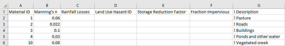
Surface roughness or bed resistance values (e.g. Manning’s n) are assigned to material IDs. In order for TUFLOW to associate the Manning’s n to the Material ID, a TUFLOW materials file is required. This can be either a text file format .tmf, or a .csv file. This tutorial model utilises the csv format.
- Copy the materials.csv file from the Module_01\Tutorial_Data folder into the Module_01\TUFLOW\model folder. As a minimum this file must contain two columns; the first being the Material ID (as specified in the GIS layer), and the second being the Manning’s n. Additional data such as loss parameters and depth varying Manning's n values (applicable for direct rainfall modelling) are covered in later modules.
- Set a global material ID for all cells by adding the following line to the TGC file:
Set Mat == 1 ! Sets all cells to a material ID of 1
- Define spatial material definition:
- Assign materials from the GIS layer to overwrite the global material at all cells that fall within the material polygons:
QGIS - SHP
Read GIS Mat == gis\2d_mat_M01_001_R.shp ! Sets material values according to attributes in the GIS layer
QGIS - GPKG
Read GIS Mat == 2d_mat_M01_001_R ! Sets material values according to attributes in the GIS layer
- Save the TGC file.

Note: As discussed in the previous sections, the order (layering) of these commands is important.
TUFLOW Boundary Control File (TBC)
In this step the TBC and Boundary Condition Database (bc_dbase) are introduced. The TBC file contains information regarding the location of boundary conditions and internal links within the model. These include, but are not limited to:
- Upstream and downstream flow boundaries
- Downstream water level boundaries
- Water sources
- Direct rainfall
- Infiltration
- 1D/2D links
- Upstream and downstream flow boundaries
Spatial Definition of Boundary Conditions
The following upstream and downstream boundaries are used in this tutorial:
- A flow vs time (QT) boundary and a source-area (SA) boundary is used for the inflows.
- A stage vs discharge (HQ) boundary is used for the outflow.
- A flow vs time (QT) boundary and a source-area (SA) boundary is used for the inflows.
Set up boundary condition layers:
TUFLOW Boundary Control File (TBC)
The boundary condition layers are read into TUFLOW in a new text file, the TBC.
- Create a new text file and save as M01_001.tbc in the Module_01\TUFLOW\model folder.
- Open the file in a text editor and add the boundary conditions:
QGIS - SHP
Read GIS BC == gis\2d_bc_M01_001_L.shp ! Reads in 2D boundaries
Read GIS SA == gis\2d_sa_M01_001_R.shp ! Reads in 2D source area boundaries
QGIS - GPKG
Read GIS BC == 2d_bc_M01_001_L ! Reads in 2D boundaries
Read GIS SA == 2d_sa_M01_001_R ! Reads in 2D source area boundaries
- Save the TBC.
TUFLOW Boundary Condition Database (bc_dbase)
The bc_dbase is a comma delimited file with .csv extension. It can be opened in any spreadsheet software or a text editor.
A hydrograph is associated with all of the upstream boundaries:
- Open the template bc database TUFLOW Tutorial Model BC Database.xlsx from the Module_01\Tutorial_Data folder.
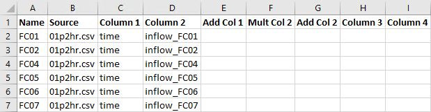
- There are two sheets in the file, 'bc_dbase' and '01p2hr'. Complete the bc_dbase worksheet:
- Enter the name of the first upstream boundary condition under the 'Name' heading. The name must appear exactly as it does in the boundary condition layer, (i.e. FC01).
- Enter the text '01p2hr.csv' under the 'Source' heading. It is a source file for TUFLOW to extract the timeseries data.
- Enter the text 'time' and 'inflow_FC01' under the 'Column 1' and 'Column 2' heading. These correspond to the data headers in the source timeseries file.
- Enter the name of the first upstream boundary condition under the 'Name' heading. The name must appear exactly as it does in the boundary condition layer, (i.e. FC01).
- Repeat the above process for all of the boundary conditions (i.e. FC02, FC04, FC05, FC06 and FC07). Note, FC02 is used in a later tutorial and Columns E to I are to remain black. The final bc_dbase should show as below:
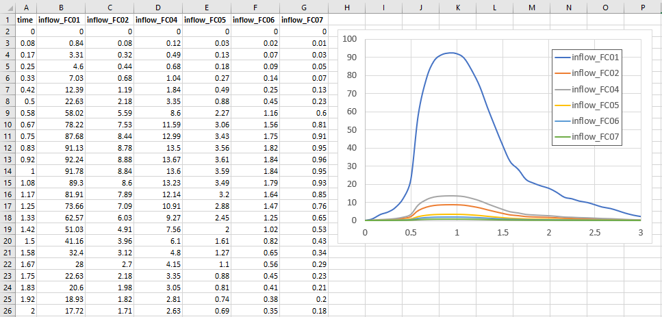
- Switch to the '01p2hr' sheet, and review the provided hydrographs. Note: the 'Inflow_FC02' hydrograph is not used in this tutorial.
- Save both of the sheets in a csv format that TUFLOW can read. In the Module_01\TUFLOW\bc_dbase directory, there should be two new files, bc_dbase.csv and 01p2hr.csv.


2D Time Series Plot Output
The 2D plot output (2d_po) objects allow for a wide range of hydraulic parameters to be output from the 2D domain as time series data at predefined locations.
TUFLOW Control File (TCF)
The TCF file references all the control files, specifies time and output controls. This is the last step before running the simulation.
- Create a new text file and save as M01_5m_001.tcf in the Module_01\TUFLOW\runs folder.
- Open the file in a text editor and add the following commands:
QGIS - SHP
! MODEL INITIALISATION
Tutorial Model == ON ! Required command to run this tutorial model licence free
GIS Format == SHP ! Specify SHP as the output format for all GIS files
SHP Projection == ..\model\gis\projection.prj ! Sets the GIS projection for the TUFLOW Model
TIF Projection == ..\model\grid\DEM.tif ! Sets the GIS projection for the output grid files
! Write Empty GIS Files == ..\model\gis\empty ! Creates template GIS layers, commented out as files were already created
QGIS - GPKG
! MODEL INITIALISATION
Spatial Database == ..\model\gis\M01_001.gpkg ! Specify the location of the GeoPackage Spatial Database
Tutorial Model == ON ! Required command to run this tutorial model licence free
GIS Format == GPKG ! Specify GPKG as the output format for all GIS files
GPKG Projection == ..\model\gis\projection.gpkg ! Sets the GIS projection for the TUFLOW Model
TIF Projection == ..\model\grid\DEM.tif ! Sets the GIS projection for the output grid files
! Write Empty GIS Files == ..\model\gis\empty ! Creates template GIS layers, commented out as files were already created
- Define the solution scheme and specify Sub-Grid Sampling (SGS) commands:
! SOLUTION SCHEME
Solution Scheme == HPC ! Heavily Parallelised Compute, uses adaptive timestepping
Hardware == GPU ! Comment out if GPU card is not available or replace with "Hardware == CPU"
SGS == ON ! Switches on Sub-Grid Sampling
SGS Sample Target Distance == 0.5 ! Sets SGS Sample Target Distance to 0.5m
For information on SGS, see Section 3.2 of the latest Release Notes)
- Update the model inputs section. These commands reference the TGC, TBC, bc_dbase and materials file created in the above steps:
! MODEL INPUTS
Geometry Control File == ..\model\M01_001.tgc ! Reference the TUFLOW Geometry Control File
BC Control File == ..\model\M01_001.tbc ! Reference the TUFLOW Boundary Conditions Control File
BC Database == ..\bc_dbase\bc_dbase.csv ! Reference the Boundary Conditions Database
Read Materials File == ..\model\materials.csv ! Reference the Materials Definition File
- Add the following time control commands:
! TIME CONTROL
Timestep == 1 ! Specifies the first 2D computational timestep of 1 second
Start Time == 0 ! Specifies a simulation start time of 0 hours
End Time == 3 ! Specifies a simulation end time of 3 hours
- Add the following output folder commands:
! OUTPUT FOLDERS
Log Folder == log ! Location of the log output files (e.g. .tlf and _messages files)
Output Folder == ..\results\ ! Location of the 2D output files and prefixes them with the .tcf filename
Write Check Files == ..\check\ ! Location of the 2D check files and prefixes them with the .tcf filename
- Add the following output settings commands:
! OUTPUT SETTINGS
Map Output Format == XMDF TIF ! Result file types
Map Output Data Types == h V d dt ! Outputs water levels, velocities, depths, minimum timestep
Map Output Interval == 300 ! Outputs map data every 300 seconds (5 minutes)
TIF Map Output Interval == 0 ! Outputs only maximums for grids
- Reference the 2d_po layers. When reading in time-series layers, such as 2d_po files, its necessary to use a Time Series Output Interval command. This command specifies the output interval in seconds for the time-series based output:
QGIS - SHP
! TIME SERIES PLOT OUTPUT
Read GIS PO == ..\model\gis\2d_po_M01_001_L.shp ! Reads in plot output line
Read GIS PO == ..\model\gis\2d_po_M01_001_P.shp ! Reads in plot output point
Time Series Output Interval == 60 ! Outputs time series data every 60 seconds
QGIS - GPKG
! TIME SERIES PLOT OUTPUT
Read GIS PO == 2d_po_M01_001_L ! Reads in plot output line
Read GIS PO == 2d_po_M01_001_P ! Reads in plot output point
Time Series Output Interval == 60 ! Outputs time series data every 60 seconds
- Save the TCF file. The TUFLOW simulation is ready to be run for the first time.
The comments (following the exclamation marks) are not required and these commands are generally self explanatory. For this tutorial model they are included to clarify the purpose of each line.
Running the Simulation
Set up a simple batch file (.bat) to run TUFLOW. This approach calls the TUFLOW executable file (.exe) and runs the TCF file.
- Create a new text file in the Module_01\TUFLOW\runs folder and save as _run_M01_HPC.bat.
- Open the _run_M01_HPC.bat in a text editor and include a file path to the executable from the exe\2026.0.0 folder and the TCF name:
"..\..\..\exe\2026.0.0\TUFLOW_iSP_w64.exe" M01_5m_001.tcf
Note: A relative path is used for the executable and the TCF, a full file path can also be used. - Save the batch file and double click it in file explorer to run the simulation.
This opens the TUFLOW console window and the simulation begins running. The simulation usually takes a few minutes to process (depending on the computer hardware). While the model is running, it is a good practise to fill out a modelling log. It includes developer notes keeping a record of TUFLOW simulations and changes from one version to the next, for more information see here. A template is included in the Module_01\Tutorial_Data folder.
If the simulation is successful, the console window should look like the image below.

Troubleshooting
See tips on common mistakes and troubleshooting steps if the model doesn't run:
Check Files
TUFLOW writes a series of check files during the model initialisation process when the Write Check Files command is specified in the TCF. The files are either in a tabular form (.csv), GIS Vector format (.gpkg, .shp, .mif) or GIS Raster format (.tif, .flt, .asc) and contain information on the input data processed by TUFLOW.
While the model is running, review the added features are specified correctly:
Results
Two map output formats specified for this tutorial:
- TIF - Grid based output format writing map output data types separately
- XMDF - Mesh based output format containing all map output data types in a single file
When the model is finished, review the results, either using TUFLOW Viewer or TUFLOW Viewer V2:
Reviewing Model Performance
There are a number of useful outputs from TUFLOW for reviewing the model performance.
TUFLOW Log File
The first place to look is in the TUFLOW Log File (TLF). The Log Folder == log command in the TCF controls where the log file is written.
Navigate to the Module_01\TUFLOW\runs\log folder and open the M01_5m_001.tlf file in a text editor. Scroll down to the bottom to 'Simulation Summary'. This includes information about the computation time, messages, volume calculations and mass error.

HPC TUFLOW Log File
As the model is using the HPC solution scheme, there is a second log file automatically written from the same command. Navigate to the Module_01\TUFLOW\runs\log folder and open the M01_5m_001.hpc.tlf file. The HPC solution scheme, by default, uses adaptive timestepping to progress through the simulation. The timestep is adjusted so it complies with the mathematical stability criteria of a 2D SWE explicit solution. This is controlled by three control numbers, further information is provided here.
Scroll down the hpc.tlf to 'iStep'. This is the point at which the model successfully compiled and began running. The three HPC control numbers are listed in the columns after time. Then the number of wet cells, the volume of water, the dt (minimum timestep) and the efficiency of the solver. As the model starts to gain wet cells dt drops, but should eventually stabilise. Similarly, model efficiency should increase as the model progresses.

Other Model Performance Indicators
For more information on how to review HPC models, see HPC Model Review.
Conclusion
- Simple 2D TUFLOW model was created with required GIS and text based inputs.
- Check files were used to review the model setup.
- Results were visualised and the performance of the model reviewed.
- For further training opportunities see TUFLOW Training Catalogue and/or contact training@tuflow.com.
- Alternatively, see the TUFLOW Example Models to explore the full list of TUFLOW features.
Increasing Model Resolution (Optional)
This section includes an optional exercise to reduce the cell size from 5m to 2.5m. Consider the impact this has on the model results and the runtime.
To reduce the cell size in the model:
- Save the TUFLOW control file M01_5m_001.tcf as M01_2.5m_001.tcf.
- Save the geometry control file M01_001.tgc as M01_2.5m_001.tgc.
- Modify the cell size in the geometry control file to '2.5' meters.
- In the TCF, update the reference to the new TGC.
- Update the batch file with the updated TCF file and run the simulation.
| Up |
|---|