TUFLOW SWMM Tutorial M02 Check QGIS: Difference between revisions
Chris Huxley (talk | contribs) |
No edit summary |
||
| (46 intermediate revisions by 4 users not shown) | |||
| Line 4: | Line 4: | ||
<ol> |
<ol> |
||
<li> |
<li>Navigate to the '''TUFLOW\results''' folder and open '''TS02_5m_001_swmm.inp''' in Notepad++. |
||
<li> |
<li>Manual Data Review (Optional): Review the Junction, Outfall, Conduit, Losses, and XSections information in the text file. |
||
</ol> |
</ol> |
||
<br> |
|||
=== QGIS Data === |
=== QGIS Data === |
||
It can be useful to review the inp file created by TUFLOW after all inp files are combined. |
|||
The QGIS TUFLOW Plugin SWMM Processing Tool, 'GeoPackage - Create from SWMM inp' can be used to create a spatial GeoPackage version of the INP data for post simulation review checking. |
|||
<ol> |
<ol> |
||
<li>In the Processing Toolbox, select 'GeoPackage - |
<li>In the Processing Toolbox, go to TUFLOW >> SWMM and select '<u>[[QGIS_SWMM_GeoPackage_Create_from_SWMM_inp |GeoPackage - Create from SWMM inp ]]</u>'. This opens the dialog shown below. |
||
:*SWMM Input File (inp): Navigate to the '''TUFLOW\results''' folder and select '''TS02_5m_001_swmm.inp'''. |
:*SWMM Input File (inp): Navigate to the '''TUFLOW\results''' folder and select '''TS02_5m_001_swmm.inp'''. |
||
:*CRS for GeoPackage: Click the drop down menu and select ‘Project CRS: EPSG:32760 - WGS 84 / UTM zone 60S’. |
:*CRS for GeoPackage: Click the drop down menu and select ‘Project CRS: EPSG:32760 - WGS 84 / UTM zone 60S’. |
||
:*SWMM Tags to ignore: leave blank. |
:*SWMM Tags to ignore: leave blank. |
||
:*GeoPackage output filename: Click the ... and select 'Save to |
:*GeoPackage output filename: Click the ... and select 'Save to File'. Navigate to the '''TUFLOW\check''' folder and set the GeoPackage output filename to '''TS02_5m_001_swmm_check.gpkg'''. |
||
<li>Click 'Run'. |
<li>Click 'Run'. Once the tool has finished, click 'Close'. |
||
<li>In Windows File Explorer, navigate to the '''TUFLOW\check''' folder and drag and drop '''TS02_5m_001_swmm_check.gpkg''' into QGIS. |
|||
<li>Once the tool has finished, click 'Close'. |
|||
<li>When prompted by QGIS, under 'Options', tick on 'Add layers to group', then select 'Add Layers' to open all layers within '''TS02_5m_001_swmm_check.gpkg'''. By default, all items in the available list should have been selected. |
|||
<li>'''TS02_5m_001_swmm_check.gpkg''' will now be available in the '''TUFLOW\check''' folder. |
|||
<br><br> |
|||
<li>In File Explorer, navigate to the '''TUFLOW\check''' folder and drag and drop '''TS02_5m_001_swmm_check.gpkg''' into QGIS. |
|||
{{Video|name=Animation_TS2_Check_01f.mp4|width=1236}} |
|||
<li>When prompted by QGIS, select 'Add Layers to open all layers within '''TS02_5m_001_swmm_check.gpkg'''. By default, all items in the available list should have been selected. |
|||
<br> |
<br> |
||
<li>Manual Data Review (Optional): Review the '''Links--Conduits''', '''Nodes--Junctions''' and '''Nodes--Outfalls''' information to verify the data matches the input values. This data represents the 1D pipe network details. |
|||
'''<<video>>''' |
|||
<br><br> |
|||
{{Video|name=Animation_TS2_Check_02e.mp4|width=1236}} |
|||
<br> |
<br> |
||
<li>Since the layers in '''TS02_5m_001_swmm_check.gpkg''' have been compared with the input layers, most of the input layers can be removed from the QGIS workspace. Remove all except the inlet usage layer, '''swmm_iu_TS02_001''', and the 2d_bc connections layer '''2d_bc_SWMM_Pipe_Network_Connections_001_L'''. |
|||
<li>Manual Review (Optional): Review the '''Link--Conduits''', '''Nodes--Junctions''' and '''Node--Outfalls''' information. This data represents the 1D pipe network details. |
|||
</ol> |
</ol> |
||
<br> |
|||
== TUFLOW Check Files == |
== TUFLOW Check Files == |
||
Open the TUFLOW check files: |
|||
<ol> |
<ol> |
||
<li>In File Explorer, navigate to the '''TUFLOW\check''' folder and drag and drop '''TS02_5m_001_Check.gpkg''' into QGIS. |
<li>In Windows File Explorer, navigate to the '''TUFLOW\check''' folder and drag and drop '''TS02_5m_001_Check.gpkg''' and '''TS02_5m_001_DEM_Z.tif''' (hold Ctrl to select multiple) into QGIS. |
||
<li>When prompted by QGIS, select ''' |
<li>When prompted by QGIS, under 'Options', tick on 'Add layers to group', then select '''TS02_5m_001_1d_to_2d_check_R''' and '''TS02_5m_001_swmm_pit_P''' (hold Ctrl to select multiple). Click 'Add Layers'. |
||
<li>Use the 'Apply TUFLOW Styles to Open Layers'. |
<li>Use the 'Apply TUFLOW Styles to Open Layers'. |
||
<li> |
<li>Style '''TS02_5m_001_DEM_Z.tif''' (the topography check file) using the same hillshade styling as '''DEM_Hillshade''': |
||
:*In the QGIS Layers Panel, right click '''DEM_Hillshade''' and select Styles > Copy Style. |
|||
:*Right Click '''TS02_5m_001_DEM_Z.tif''' and select Styles > Paste Style. |
|||
<li>In the QGIS Layers Panel, move the '''TS02_5m_001_DEM_Z.tif''' layer below the other check files so that the other datasets are visible. |
|||
<br><br> |
|||
{{Video|name=Animation_TS2_Check_03e.mp4|width=1236}} |
|||
<br> |
|||
</ol> |
</ol> |
||
Manual Data Review (Optional): Compare the 2D check files information against the the 1D check files to verify the model design is as intended. |
|||
'''<<video>>''' |
|||
<ol> |
|||
<li>How does the the pipe network invert elevations ('''Nodes--Junctions''') compare to the the pit inlet (surface) elevations? |
|||
<br> |
|||
</ol> |
|||
<br> |
|||
== Inlet 1D/2D Connection Refinement == |
|||
Manual Data Review (Optional): Compare the 2D check files information against the the 1D check files to verify the model design is as intended. For example: |
|||
Currently, the underground stormwater pipe network inlets are set to use the 2D cell each inlet point is contained within for the connection to the 2D domain. This is often sufficient in many models, further refinement is however possible, particularly for on-grade inlets. On-grade inlets divert a portion of the flow going past an inlet into the pipe network based on a few factors, such as approach flow (the discharge flowing down the side of the roadway), velocity, and the inlet characteristics. To obtain an accurate estimation of the approach flow in the model, the 1D/2D connection cells must extend across the area conveying flow. Most urban areas have crowned roads, in this scenario the connected cells should extend to the center of the roadway. The geometry in this example model is simplified with flow generally only on one side of the street. |
|||
To check that on-grade inlets have a sufficient number of connected 2D cells: |
|||
# How does the the pipe network invert elevations ('''Nodes--Junctions)''' compare to the the pit inlet (surface) elevations. |
|||
# Do the SWMM values for the Ysur and Apond at the pit inlet and closed junction locations vary? Do they match the values we specified when constructing the model? |
|||
== TUFLOW Pipe Integrity Tool == |
|||
Some of the optional manual data review exercises suggested in the previous sections can be carried out more easily using the visual profile plot tools included in the QGIS TUFLOW Plugin Pipe Integrity Toolkit. |
|||
<ol> |
<ol> |
||
<li>In the QGIS Layers Panel, ensure '''swmm_iu_TS02_001''' is at the top of the list. This will ensure the data within this layer is displayed above all other layers in the project. |
|||
<li>From the TUFLOW plugin, open the 1D Integrity tool.<br>[[File: integrity_tool_in_toolbar.PNG]].<br> |
|||
<li>Right click '''swmm_iu_TS02_001''' and select 'Properties'. |
|||
<li>In the 'Symbology' tab, click the top drop down menu and select 'Categorized'. |
|||
<li>To select the 'Value', click the drop down menu and select 'Placement'. |
|||
<li>Click 'Classify'. This will categorize the inlets in '''swmm_iu_TS02_001''' by their placement field and force each category to use a different color. There should be two categories: 'ON_GRADE' and 'ON_SAG'. |
|||
<li>Click 'Apply' and 'OK'. |
|||
<li>Ensure there are three 'ON_GRADE' inlets and nine 'ON_SAG' inlets. |
|||
<li>In the QGIS Layers Panel, right click '''Nodes--Junctions''' and select 'Show Labels'. This should indicate that the three on-grade inlets are 'Pit7', 'Pit9', and 'Pit15'. |
|||
<br><br> |
|||
{{Video|name=Animation_TS2_Check_Inlet_01b.mp4|width=1236}} |
|||
<br> |
|||
<li>Use the '''TS02_5m_001_1d_to_2d_check_R''' layer to compare the width of the 1D/2D connection cells with the roadway widths in the DEM. It should be clear that the cells cover less than half of the roadways and may not represent the full flow-width that we are interested in. |
|||
</ol> |
</ol> |
||
<br> |
|||
The resulting dialogue will pop up. The numbered fields are described below.<br> |
|||
There are two approaches to connect an inlet to multiple cells: |
|||
<ol> |
<ol> |
||
<li>Within the inlet usage layer, '''swmm_iu_TS02_001''', the number of connected cells is determined by the 'Conn_width' field. Increasing the connection width will select multiple cells. Note that a negative value will specify an exact number of cells regardless of the cell size. The default approach for selecting additional cells depends on whether the inlet is on-grade or on-sag. The details of the algorithm can be found in the <u>[https://docs.tuflow.com/classic-hpc/manual/latest/ TUFLOW Manual]</u>. |
|||
[[File:integrity_tool_overview.PNG]]<br> |
|||
<li>Manually specify the cells to connect using an SX connection (polyline or polygon) and CN line to the inlet location. Note this method requires removing the 'Conn1D_2D' attribute from the inlet usage layer. |
|||
<br>'''1. Input Network Lines''' - Select '''Link--Conduits'''. Use dropdown box and '+' button to add layers as inputs to tool.<br>'''2. Input Network Points''' - Select '''Nodes--Junctions''' and '''Node--Outfalls'''. Use dropdown box and '+' button to add layers as inputs to tool.<br>'''3. Input Tables''' - Not used for SWMM data review.<br>'''4. Input DEM''' - Select '''TS02_5m_001_DEM_Z'''.<br>'''5. Tool Selection''' - The active tab will determine the active tool. See [[#Tool_Documentation|Tool Documentation]] for information on each tool.<br>'''6. Status Bar''' - Contains the progress bar and status of the integrity tool. Includes information such as the current active task being performed (if one of the tools is running), and the status of the previously run tool.<br>'''7. Run''' - Runs the currently active tool (active tool determined by the current active tool tab - prior to plugin version 3.2 a radio button was used to select the active tool). |
|||
</ol> |
|||
<br> |
<br> |
||
For this model, the first option (increasing the number of cells) will be used for 'Pit9', and the second option (create manual connections) will be used for 'Pit7' and 'Pit15'. |
|||
:'''Note:''' When using the automatic method, the actual 1D/2D connected cells should be verified. |
|||
<br> |
<br> |
||
Make the following changes to the inlet usage layer: |
|||
The following example demonstrates use of the Flow Trace tool to create a profile plot for visual review of the 1D pipe network data input. |
|||
<ol> |
|||
<li>In the QGIS Layers Panel, select (left click) '''swmm_iu_TS02_001''' and toggle on editing. |
|||
<li>Use the 'Select Features' tool to highlight the inlets on the junction nodes, 'Pit7' and 'Pit15' (hold Shift to select multiple). |
|||
<li>Right click '''swmm_iu_TS02_001''' and select 'Open Attribute Table'. |
|||
<li>Clear the 'Conn1D_2D' attributes for the inlets representing 'Pit7' and 'Pit15'. |
|||
<li>For the inlet associated with 'Pit9', specify a value of -2 for the 'Conn_width'. This will connect the inlet to exactly two cells regardless of the cell size. |
|||
<li>Turn off editing to save the edits. |
|||
<br><br> |
|||
{{Video|name=Animation_TS2_Check_Inlet_03b.mp4|width=1236}} |
|||
<br> |
|||
</ol> |
|||
Next, the manual connections for 'Pit7' and 'Pit15' must be added. To save time, a 2d_bc layer with these connections has been provided. |
|||
<ol> |
|||
<li>If the QGIS Browser Panel is not already open, right click anywhere in the QGIS Toolbar Panel and tick on 'Browser Panel' from the 'Panels' options. |
|||
<li>In the QGIS Browser Panel, in the 'Project Home' directory, navigate to the '''TUFLOW_SWMM_Module_02\Tutorial_Data''' folder. |
|||
<li>Drag the '''2d_bc_SWMM_Inlet_Connections_001_L''' layer from the '''Urban_Development.gpkg''' and drop it into the '''TS02_001.gpkg''' contained within the '''TUFLOW_SWMM_Module_02\TUFLOW\model\gis''' folder. |
|||
<br><br> |
|||
{{Video|name=Animation_TS2_Check_Inlet_04b.mp4|width=1236}} |
|||
<br> |
<br> |
||
</ol> |
|||
Update the TBC: |
|||
'''<<video>>''' |
|||
<ol> |
|||
<li>Navigate to the '''TUFLOW\model''' folder and open ''' TS02_001.tbc''' in Notepad++. |
|||
<li>Add the following command to the end of the file: |
|||
:<font color="blue"><tt>Read GIS BC</tt></font> <font color="red"><tt>== </tt></font> <font color="black"><tt>2d_bc_SWMM_Inlet_Connections_001_L</tt></font> <font color="green"><tt> ! Reference the TUFLOW BC File</tt></font><br> |
|||
</ol> |
</ol> |
||
<br> |
|||
Rerun the model and review the check files to verify that the on-grade inlets are now connected to multiple cells. |
|||
<br> |
|||
== TUFLOW Pipe Integrity Tool == |
|||
Some of the optional manual data review exercises suggested in the previous sections can be easily carried out using the QGIS TUFLOW Plugin 'Pipe Integrity Toolkit', specifically the visual profile plot tools. |
|||
<ol> |
|||
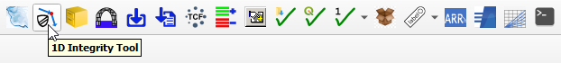
<li>Open the '1D Integrity Tool' from the TUFLOW Plugin toolbar. |
|||
<br><br> |
|||
[[File:tuflow_plugin_1D_integrity.png]] |
|||
<br><br> |
|||
<li>The resulting dialog will appear. |
|||
<br><br> |
|||
[[File:1D_Integrity_dialog_2.png]] |
|||
<br><br> |
|||
<li>Set up the tool for this model: |
|||
:*Input Network Lines: Use the dropdown box and select '''TS02_5m_001_swmm_check >> Links--Conduits'''. Click the '+' button to add the layer as an input to the tool. |
|||
:*Input Network Points: Using the same process as above, add '''TS02_5m_001_swmm_check >> Nodes--Junctions''' and '''TS02_5m_001_swmm_check >> Nodes--Outfalls''' to the tool. |
|||
:*Input Tables: Leave blank as it is not used for SWMM data review. |
|||
:*Input DEM: Tick on and use the dropdown box to select '''TS02_5m_001_DEM_Z'''. |
|||
</ol> |
|||
'''Note:''' For further information on the 1D Integrity Tool and its functionality, see <u>[[1D Integrity Tool|1D Integrity Tool]]</u>. |
|||
<br><br> |
|||
<ol> |
|||
{{Video|name=Animation_TS2_Check_04e.mp4|width=1350}} |
|||
<br> |
|||
</ol> |
|||
The following example demonstrates the 'Flow Trace' tool. It will be used to create a profile plot for visual review of the 1D pipe network data input. |
|||
<ol> |
|||
<li>In the QGIS Layers Panel, right click '''Links--Conduits''' and select 'Zoom to Layer(s)'. |
|||
<li>Use the 'Select Features' tool to select conduit 'Pipe6'. |
|||
<li>At the bottom of the 1D Integrity tool dialog, there is a list of tools. Select the 'Flow Trace' tab. |
|||
<li>Enter the following options: |
|||
<br><br> |
|||
[[File:1D_Integrity_flow_trace_options.png]] |
|||
<br><br> |
|||
<li>Click 'Run'. |
|||
<li>The tool will select all the upstream conduits and also add another output layer identifying the locations which fail the flow area and invert checks. |
|||
<li>A Flow Trace window will appear. It provides a 'long plot' of the long sections of the various upstream paths from the selected conduit, highlighting the areas of continuity failures. The plot should be consistent with the output GIS layer that is also generated by the flow trace tool. |
|||
<br><br> |
|||
{{Video|name=Animation_TS2_Check_05e.mp4|width=1350}} |
|||
<br> |
|||
</ol> |
|||
<br><br> |
|||
{{Tips Navigation |
{{Tips Navigation |
||
Latest revision as of 09:56, 23 September 2024
SWMM Check Files
Text Data
When TUFLOW runs SWMM, it can accommodate for multiple INP input files within the SWMM Control file. TUFLOW combines the input INP files into a single combined INP file for the simulation execution. The combined file TUFLOW uses is written to the TUFLOW\results folder.
- Navigate to the TUFLOW\results folder and open TS02_5m_001_swmm.inp in Notepad++.
- Manual Data Review (Optional): Review the Junction, Outfall, Conduit, Losses, and XSections information in the text file.
QGIS Data
It can be useful to review the inp file created by TUFLOW after all inp files are combined.
- In the Processing Toolbox, go to TUFLOW >> SWMM and select 'GeoPackage - Create from SWMM inp '. This opens the dialog shown below.
- SWMM Input File (inp): Navigate to the TUFLOW\results folder and select TS02_5m_001_swmm.inp.
- CRS for GeoPackage: Click the drop down menu and select ‘Project CRS: EPSG:32760 - WGS 84 / UTM zone 60S’.
- SWMM Tags to ignore: leave blank.
- GeoPackage output filename: Click the ... and select 'Save to File'. Navigate to the TUFLOW\check folder and set the GeoPackage output filename to TS02_5m_001_swmm_check.gpkg.
- Click 'Run'. Once the tool has finished, click 'Close'.
- In Windows File Explorer, navigate to the TUFLOW\check folder and drag and drop TS02_5m_001_swmm_check.gpkg into QGIS.
- When prompted by QGIS, under 'Options', tick on 'Add layers to group', then select 'Add Layers' to open all layers within TS02_5m_001_swmm_check.gpkg. By default, all items in the available list should have been selected.
- Manual Data Review (Optional): Review the Links--Conduits, Nodes--Junctions and Nodes--Outfalls information to verify the data matches the input values. This data represents the 1D pipe network details.
- Since the layers in TS02_5m_001_swmm_check.gpkg have been compared with the input layers, most of the input layers can be removed from the QGIS workspace. Remove all except the inlet usage layer, swmm_iu_TS02_001, and the 2d_bc connections layer 2d_bc_SWMM_Pipe_Network_Connections_001_L.
TUFLOW Check Files
Open the TUFLOW check files:
- In Windows File Explorer, navigate to the TUFLOW\check folder and drag and drop TS02_5m_001_Check.gpkg and TS02_5m_001_DEM_Z.tif (hold Ctrl to select multiple) into QGIS.
- When prompted by QGIS, under 'Options', tick on 'Add layers to group', then select TS02_5m_001_1d_to_2d_check_R and TS02_5m_001_swmm_pit_P (hold Ctrl to select multiple). Click 'Add Layers'.
- Use the 'Apply TUFLOW Styles to Open Layers'.
- Style TS02_5m_001_DEM_Z.tif (the topography check file) using the same hillshade styling as DEM_Hillshade:
- In the QGIS Layers Panel, right click DEM_Hillshade and select Styles > Copy Style.
- Right Click TS02_5m_001_DEM_Z.tif and select Styles > Paste Style.
- In the QGIS Layers Panel, move the TS02_5m_001_DEM_Z.tif layer below the other check files so that the other datasets are visible.
Manual Data Review (Optional): Compare the 2D check files information against the the 1D check files to verify the model design is as intended.
- How does the the pipe network invert elevations (Nodes--Junctions) compare to the the pit inlet (surface) elevations?
Inlet 1D/2D Connection Refinement
Currently, the underground stormwater pipe network inlets are set to use the 2D cell each inlet point is contained within for the connection to the 2D domain. This is often sufficient in many models, further refinement is however possible, particularly for on-grade inlets. On-grade inlets divert a portion of the flow going past an inlet into the pipe network based on a few factors, such as approach flow (the discharge flowing down the side of the roadway), velocity, and the inlet characteristics. To obtain an accurate estimation of the approach flow in the model, the 1D/2D connection cells must extend across the area conveying flow. Most urban areas have crowned roads, in this scenario the connected cells should extend to the center of the roadway. The geometry in this example model is simplified with flow generally only on one side of the street.
To check that on-grade inlets have a sufficient number of connected 2D cells:
- In the QGIS Layers Panel, ensure swmm_iu_TS02_001 is at the top of the list. This will ensure the data within this layer is displayed above all other layers in the project.
- Right click swmm_iu_TS02_001 and select 'Properties'.
- In the 'Symbology' tab, click the top drop down menu and select 'Categorized'.
- To select the 'Value', click the drop down menu and select 'Placement'.
- Click 'Classify'. This will categorize the inlets in swmm_iu_TS02_001 by their placement field and force each category to use a different color. There should be two categories: 'ON_GRADE' and 'ON_SAG'.
- Click 'Apply' and 'OK'.
- Ensure there are three 'ON_GRADE' inlets and nine 'ON_SAG' inlets.
- In the QGIS Layers Panel, right click Nodes--Junctions and select 'Show Labels'. This should indicate that the three on-grade inlets are 'Pit7', 'Pit9', and 'Pit15'.
- Use the TS02_5m_001_1d_to_2d_check_R layer to compare the width of the 1D/2D connection cells with the roadway widths in the DEM. It should be clear that the cells cover less than half of the roadways and may not represent the full flow-width that we are interested in.
There are two approaches to connect an inlet to multiple cells:
- Within the inlet usage layer, swmm_iu_TS02_001, the number of connected cells is determined by the 'Conn_width' field. Increasing the connection width will select multiple cells. Note that a negative value will specify an exact number of cells regardless of the cell size. The default approach for selecting additional cells depends on whether the inlet is on-grade or on-sag. The details of the algorithm can be found in the TUFLOW Manual.
- Manually specify the cells to connect using an SX connection (polyline or polygon) and CN line to the inlet location. Note this method requires removing the 'Conn1D_2D' attribute from the inlet usage layer.
For this model, the first option (increasing the number of cells) will be used for 'Pit9', and the second option (create manual connections) will be used for 'Pit7' and 'Pit15'.
- Note: When using the automatic method, the actual 1D/2D connected cells should be verified.
Make the following changes to the inlet usage layer:
- In the QGIS Layers Panel, select (left click) swmm_iu_TS02_001 and toggle on editing.
- Use the 'Select Features' tool to highlight the inlets on the junction nodes, 'Pit7' and 'Pit15' (hold Shift to select multiple).
- Right click swmm_iu_TS02_001 and select 'Open Attribute Table'.
- Clear the 'Conn1D_2D' attributes for the inlets representing 'Pit7' and 'Pit15'.
- For the inlet associated with 'Pit9', specify a value of -2 for the 'Conn_width'. This will connect the inlet to exactly two cells regardless of the cell size.
- Turn off editing to save the edits.
Next, the manual connections for 'Pit7' and 'Pit15' must be added. To save time, a 2d_bc layer with these connections has been provided.
- If the QGIS Browser Panel is not already open, right click anywhere in the QGIS Toolbar Panel and tick on 'Browser Panel' from the 'Panels' options.
- In the QGIS Browser Panel, in the 'Project Home' directory, navigate to the TUFLOW_SWMM_Module_02\Tutorial_Data folder.
- Drag the 2d_bc_SWMM_Inlet_Connections_001_L layer from the Urban_Development.gpkg and drop it into the TS02_001.gpkg contained within the TUFLOW_SWMM_Module_02\TUFLOW\model\gis folder.
Update the TBC:
- Navigate to the TUFLOW\model folder and open TS02_001.tbc in Notepad++.
- Add the following command to the end of the file:
- Read GIS BC == 2d_bc_SWMM_Inlet_Connections_001_L ! Reference the TUFLOW BC File
- Read GIS BC == 2d_bc_SWMM_Inlet_Connections_001_L ! Reference the TUFLOW BC File
Rerun the model and review the check files to verify that the on-grade inlets are now connected to multiple cells.
TUFLOW Pipe Integrity Tool
Some of the optional manual data review exercises suggested in the previous sections can be easily carried out using the QGIS TUFLOW Plugin 'Pipe Integrity Toolkit', specifically the visual profile plot tools.
- Open the '1D Integrity Tool' from the TUFLOW Plugin toolbar.
- The resulting dialog will appear.
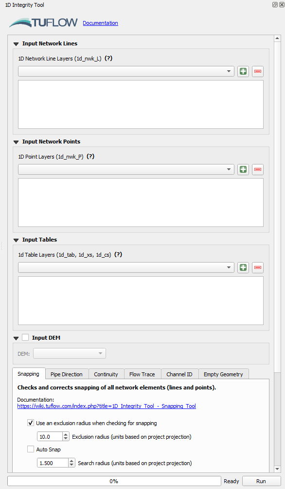
- Set up the tool for this model:
- Input Network Lines: Use the dropdown box and select TS02_5m_001_swmm_check >> Links--Conduits. Click the '+' button to add the layer as an input to the tool.
- Input Network Points: Using the same process as above, add TS02_5m_001_swmm_check >> Nodes--Junctions and TS02_5m_001_swmm_check >> Nodes--Outfalls to the tool.
- Input Tables: Leave blank as it is not used for SWMM data review.
- Input DEM: Tick on and use the dropdown box to select TS02_5m_001_DEM_Z.


Note: For further information on the 1D Integrity Tool and its functionality, see 1D Integrity Tool.
The following example demonstrates the 'Flow Trace' tool. It will be used to create a profile plot for visual review of the 1D pipe network data input.
- In the QGIS Layers Panel, right click Links--Conduits and select 'Zoom to Layer(s)'.
- Use the 'Select Features' tool to select conduit 'Pipe6'.
- At the bottom of the 1D Integrity tool dialog, there is a list of tools. Select the 'Flow Trace' tab.
- Enter the following options:
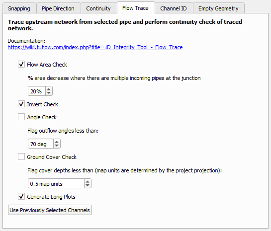
- Click 'Run'.
- The tool will select all the upstream conduits and also add another output layer identifying the locations which fail the flow area and invert checks.
- A Flow Trace window will appear. It provides a 'long plot' of the long sections of the various upstream paths from the selected conduit, highlighting the areas of continuity failures. The plot should be consistent with the output GIS layer that is also generated by the flow trace tool.

| Up |
|---|