FMA Challenge 3: Difference between revisions
Anne.Kolega (talk | contribs) m →Open Boundaries: i.e. |
|||
| (66 intermediate revisions by 5 users not shown) | |||
| Line 1: | Line 1: | ||
= Introduction = |
= Introduction = |
||
This demo comprises the third and final model of the FMA Challenge series and assumes that you're an intermediate to advanced TUFLOW user. <br> |
|||
In this challenge, a typical non-urban stream of the California Central Valley will be explored. The stream originates near the Sierra Nevada Foothills and conveys runoff to the West into the Central Valley Flood Management System. The streams are natural, with large amounts of conveyance in their upper reaches. As the streams progress downstream, their conveyance capacity gradually reduces. At some point nearing the valley floor, typical levees have been constructed to contain normal floods within the conveyance systems. |
|||
This challenge investigates a typical non-urban stream from the California Central Valley. The stream originates near the Sierra Nevada Foothills and conveys runoff to the West into the Central Valley Flood Management System. The streams are natural, with large amounts of conveyance in their upper reaches. As the streams progress downstream, their conveyance capacity gradually reduces. At some point nearing the valley floor, levees have been constructed in an effor to maintain flooding to within the the main flow conveyance area. |
|||
From this challenge, it is expected you will develop skills in:<br> |
From this challenge, it is expected you will develop skills in:<br> |
||
*Understanding of the influence of levees on flood behaviour; |
*Understanding of the influence of levees on flood behaviour; |
||
*Understanding of the influence of channel roughness on flood behaviour; |
|||
*Understanding of the influence of infiltration on flood behaviour; |
*Understanding of the influence of infiltration on flood behaviour; |
||
*Nested 1D/2D models; and |
*Nested 1D/2D models; and |
||
*Understanding the Green and Ampt infiltration method and USDR soil types. |
*Understanding the Green and Ampt infiltration method and USDR soil types.<br> |
||
Data for this model is provided via external hard drive or DVD. |
|||
==Relevant Tutorials== |
|||
It may be useful to revisit some of the following tutorials:<br> |
|||
*<font color="blue"><tt>1D-2D Linking</tt></font>- [[Tutorial Module02|Tutorial Module 2]] |
|||
*<font color="blue"><tt>Running Events and Scenarios</tt></font>- http://www.tuflow.com/forum/index.php?showtopic=1149&hl=scenario |
|||
==Information to Modelers== |
|||
Assignment of all parameters for this analysis are at the discretion of the modeler. A high resolution aerial image is provided so that land cover details can be inspected. Information on the problem definition can be found on '''FMA_Challenge_Models/FMA_Scenario3/FMA_Challenge_Model_Introductions'''.<br> |
|||
=Relevant Files= |
|||
It is up to the modeler's discretion to determine what GIS package to use, what text editor to use, and how to run their models (batch mode or within the text editor).All relevant files can be found on '''FMA_Challenge_Models/FMA_Scenario3/''' |
|||
DData for this model is provided in a variety of different GIS compatible formats. Download the dataset that matches the GIS software you are using: |
|||
=Solution to Challenge 3= |
|||
*[https://www.tuflow.com/Download/TUFLOW/Demo_Models/FMA_Challenge_Model_3_QGIS.zip QGIS Data Download] |
|||
A sample solution has been presented, courtesy of BMT WBM. |
|||
*[https://www.tuflow.com/Download/TUFLOW/Demo_Models/FMA_Challenge_Model_3_Mapinfo.zip MapInfo Data Download] |
|||
*[https://www.tuflow.com/Download/TUFLOW/Demo_Models/FMA_Challenge_Model_3_ArcGIS.zip ArcGIS Data Download] |
|||
=Relevant Tutorials= |
|||
==Cross Section Spacing, Grid Size, Mesh Element Size, and Effects of Hydraulic Structures== |
|||
Other tutorials that are relevant to this challenge that may help refresh your memory are as follows:<br> |
|||
The model was set up as a TUFLOW 1D/2D model. Two different resolutions for the floodplain were simulated using 100ft and 200ft cell sizes. |
|||
*1D-2D Linking - <u>[[Tutorial_M03|Tutorial Module 3]]</u> |
|||
*1D Nested Channel - <u>[[Tutorial_M11|Tutorial Module 11]]</u> |
|||
*Running Scenarios - <u>[[Tutorial_M08|Tutorial Module 8]]</u> |
|||
*Running Events - <u>[[Tutorial_M09|Tutorial Module 09]]</u> |
|||
<br> |
|||
=Model Setup= |
|||
1D sections spacing were generally between 500ft and 1000ft (except at structures). Structures were modeled with additional energy loss, to simplify the model a value of 1.0 V2/2g was used for all structures in the main creek. |
|||
This section provides an overview and discussion of the model domain setup. |
|||
It is at your discretion which GIS package, text editor and method of model simulation to use (batch mode or within the text editor). All files required to setup and run the models are available within the download package. You have the choice of running with shape file or mif for usage in ArcGIS/QGIS or Mapinfo respectively. This model does not require a licence dongle to run. |
|||
==Cross Sections, Grid Setup and Cell Size== |
|||
Linking between 1D/2D was along the top of the levees. |
|||
The model is set up as a TUFLOW 1D/2D model. The 2D domain is modelled using 100ft (~30.5m) and 200ft (~60.96m) cell sizes. |
|||
Cell size selection is managed through the use of variables. |
|||
Within the river bed, 1D sections spacing are generally between 500ft and 1000ft. The exception is at structures where more frequent sections are necessary to adequately model changes in flow width and velocity in these areas.<br> |
|||
All outflow from the model was assumed to be only via the main creek (ie. there was no water level boundary applied to the 2D overbank domain). |
|||
The number of cross sections, grids, or mesh elements used were as follows:<br> |
|||
{| align="center" class="wikitable" width="50%" |
{| align="center" class="wikitable" width="50%" |
||
| Line 42: | Line 39: | ||
! style="background-color:#005581; font-weight:bold; color:white;"| Active 2D Cells |
! style="background-color:#005581; font-weight:bold; color:white;"| Active 2D Cells |
||
|- |
|- |
||
| 100ft || 338, |
| 100ft || 338,020 |
||
|- |
|- |
||
| 200ft || 84, |
| 200ft || 84,818 |
||
|} |
|} |
||
==Computational Domain Assembly and Execution== |
|||
==Topography and Bed Resistance== |
|||
The provided DEM via GMG format was too coarse for hydraulic modeling as key hydraulic features (such as levee crests) were not adequately represented. The first step was therefore to process the 20Gb of LiDAR data into a higher resolution DEM. A 10ft DEM was created, a small part of which is illustrated below. |
The provided DEM via GMG format was too coarse for hydraulic modeling as key hydraulic features (such as levee crests) were not adequately represented. The first step was therefore to process the 20Gb of LiDAR data into a higher resolution DEM. A 10ft DEM was created, a small part of which is illustrated below. |
||
| Line 77: | Line 75: | ||
|} |
|} |
||
To check these Manning's 'n' assumptions, a sensitivity testing was completed on the in-bank roughness and is detailed further in the following sections. |
|||
==Boundary Conditions== |
|||
The 1d/2d linking was along the top of the levee. The elevations along these levees were extracted from the 10ft DEM, these and other significant features were included in the TUFLOW model as 3D GIS breakline layers, ensuring the hydraulic control is represented in the grid regardless of cell size. |
|||
===Open Boundaries=== |
|||
The flood extent from the 100ft 2D grid model is shown below. |
|||
A single hydrograph, derived from a previous hydrologic analysis was applied as a QT boundary via a 1d_bc. |
|||
All outflow from the model was assumed to be only via the main channel (i.e. there was no water level boundary applied to the 2D overbank domain). |
|||
===1D/2D Linking=== |
|||
[[File:FMA3_3.jpg|600px]] |
|||
The 1D river channel model was linked to the 2D model using HX cells along the top of either natural or build levees on either side of the channel. These locations defined the location of spill into the floodplain and are the key control on how much flow can interact between the floodplain and river conveyance area. The elevations along these levees were extracted from the 10ft DEM, and other significant features were included in the TUFLOW model as 3D GIS breakline layers, ensuring the hydraulic control is represented in the grid regardless of cell size. |
|||
=Results - No Infiltration= |
|||
===Sensitivity Creek Manning's n Test (Scenario 100ft n0.1) |
|||
The flood extent from the 100ft 2D grid model with no infiltration and Manning's 'n' within the channel of 0.2 is shown below. |
|||
As discussed in the Manning’s n table above, the main creek n value of 0.20 is considered very high, especially in the lower reaches of the study area. A sensitivity analysis was carried out by lowering all the Manning’s n values in the main channel (modeled as 1D cross-sections) to 0.10. |
|||
The image below shows the flood depths and extent, and the outflow is included in the ftp download. Of particular interest is that reducing the n value to 0.1 has a significant effect on the arrival time of the flood waters at the model outlet (much earlier), and reduces the volume of water flowing onto the floodplain by around 20% due to the higher conveyance of the creek. Also of interest is that for the n=0.2 scenario, some overbank floodwaters return to the main creek near the model outlet causing a delayed second rise in the outlet flow hydrographs as illustrated in the chart further below. This effect does not occur for the n=0.1 scenario, with all overbank floodwaters remaining on the floodplain. |
|||
[[File: |
[[File:FMA3_3.jpg|600px]] |
||
[[File:FMA3_5.jpg|600px]] |
|||
'''Chart of flow out of the model for the different scenarios simulated. Note that “100ft GA” is the infiltration scenario modeled for Challenge 3+.''' |
|||
The sections of levee that were overtopped were post-processed using GIS for the 100ft with n=0.2 scenario as illustrated by the magenta lines in the image below. The GIS layer showing the overtopped sections is provided as part of the ftp download. |
|||
==Levee Overtopping Assessment== |
|||
To assess the timing and location of where levee banks were overtopped, the TGC was setup with the evacuation route command:<br> <font color="blue"><tt>Read GIS Z Shape Route </tt></font> <font color="red"><tt>==</tt></font> shp\2d_zshr_T3_levees_001_L.shp | shp\2d_zsh_T3_levees_001_P.shp.<br> |
|||
Via review of the RC Map Output Data Type and the _RCP output point layer we can identify sections of the levee where a breach has occured (refer below).<br> |
|||
[[File:FMA3_6.jpg|600px]] |
[[File:FMA3_6.jpg|600px]] |
||
==Sensitivity Creek Manning's n Test (Scenario 100ft n0.1)== |
|||
As discussed in the Manning’s n table above, the main creek n value of 0.20 is considered very high, especially in the lower reaches of the study area. A sensitivity analysis was carried out by lowering all the Manning’s n values in the main channel (modelled as 1D cross-sections) to 0.10. |
|||
The image below shows the flood depths and extent for the two non-infiltration simulations at 100ft resolution (left with channel 'n' = 0.2, right with channel 'n' = 0.1). Some significant deviations in flood extent can be observed, particularly south of the main channel. This can be largely attributed to the higher conveyance in the channel for the 'n'=0.1 case. <br> |
|||
[[File:FMA3_3.jpg|600px]][[File:FMA3_4.jpg|600px]]<br> |
|||
The effect of channel roughness can also be seen in hydrograph outflows from the model downstream boundary (refer figure below). |
|||
Of particular interest is that reducing the n value to 0.1 has a significant effect on the arrival time of the flood waters at the model outlet (much earlier), and reduces the volume of water flowing onto the floodplain by around 20% due to the higher conveyance of the creek. Also of interest is that for the n=0.2 scenario, some overbank floodwaters return to the main creek near the model outlet causing a delayed second rise in the outlet flow hydrographs as illustrated in the chart further below. This effect does not occur for the n=0.1 scenario, with all overbank floodwaters remaining on the floodplain.<br> |
|||
Please note the scenarios provided in the legend below are as follows:<br> |
|||
*100ft = 100ft cell resolution, no infiltration and channel roughness of 'n' = 0.2<br> |
|||
*200ft = 200ft cell resolution, no infiltration and channel roughness of 'n' = 0.2<br> |
|||
*100ft (n0.1) = 100ft cell resolution, no infiltration and channel roughness of 'n' = 0.1<br> |
|||
*100ft GA = 100ft cell resolution, Green and Ampt infiltration with channel roughness of 'n' = 0.2<br> |
|||
*Inflow = Hydrograph input at northeastern QT boundary.<br> |
|||
[[File:FMA3_5.jpg|600px]] |
|||
=Green and Ampt Infiltration Setup= |
|||
=Solution to Challenge 3+= |
|||
Where unstated, the same parameters were used as per Challenge 3. |
|||
==Computational Domain Assembly and Execution== |
|||
The 100ft and 200ft models were used from Challenge 3 with the Creek Manning’s n value set to 0.2. |
|||
Provided soils layers were roughly classified into two soil types for the purposes of demonstrating the Green-Ampt infiltration feature in TUFLOW. The soils are shown in the image below where: |
|||
<ol> |
<ol> |
||
<li>Red indicates a Sandy Loam. |
<li>Red indicates a Sandy Loam. |
||
| Line 137: | Line 140: | ||
[[File:FMA3_7.jpg|600px]] |
[[File:FMA3_7.jpg|600px]] |
||
The 100ft and 200ft simulations were re-run with |
The 100ft and 200ft simulations were re-run with Green-Ampt infiltration switched on. The resulting peak flood depths map for the 100ft simulation is shown in the image below (right) whilst the 100ft without infiltration is provided on the right. As can be seen, the extent of inundation is significantly reduced with floodwaters infiltrating before reaching the model extents or returning to the main channel. |
||
The mass balance reporting from TUFLOW indicates over half (58%) of the water infiltrates into the ground during the 171 hour simulation. For the flow out of the model see “100ft GA” in the chart of flow out of the model presented in Challenge 3. |
|||
The mass balance reporting from TUFLOW indicates over half (58%) of the water infiltrates into the ground during the 171 hour simulation. This reduction in volume can also be observed via the “100ft GA” flow hydrograph show above. |
|||
[[File:FMA3_8.jpg|600px]] |
|||
[[File:FMA3_3.jpg|600px]][[File:FMA3_8.jpg|600px]] |
|||
==Challenges== |
|||
The soils GIS layers were difficult to work with. There is a lot of detail, but no clear way to correlate the different soils with Green-Ampt parameters (porosity, hydraulic conductivity, suction, etc). |
|||
=Conclusion= |
=Conclusion= |
||
| Line 150: | Line 150: | ||
In this challenge, we explored typical non-urban stream of the California Central Valley, with scenarios of various infiltration and flood levees adopted. From this, we gained a better understanding of the influence of flood levees on surface water behaviour, understanding of the Green Ampt infiltration method and USDR soil types, and a better understanding of nested 1D/2D models. |
In this challenge, we explored typical non-urban stream of the California Central Valley, with scenarios of various infiltration and flood levees adopted. From this, we gained a better understanding of the influence of flood levees on surface water behaviour, understanding of the Green Ampt infiltration method and USDR soil types, and a better understanding of nested 1D/2D models. |
||
Congratulations on finishing |
Congratulations on finishing the FMA Demo Model 3. Please click here to return the [[Main_Page| Wiki Main Page]]. |
||
Latest revision as of 11:56, 2 April 2026
Introduction
This demo comprises the third and final model of the FMA Challenge series and assumes that you're an intermediate to advanced TUFLOW user.
This challenge investigates a typical non-urban stream from the California Central Valley. The stream originates near the Sierra Nevada Foothills and conveys runoff to the West into the Central Valley Flood Management System. The streams are natural, with large amounts of conveyance in their upper reaches. As the streams progress downstream, their conveyance capacity gradually reduces. At some point nearing the valley floor, levees have been constructed in an effor to maintain flooding to within the the main flow conveyance area.
From this challenge, it is expected you will develop skills in:
- Understanding of the influence of levees on flood behaviour;
- Understanding of the influence of channel roughness on flood behaviour;
- Understanding of the influence of infiltration on flood behaviour;
- Nested 1D/2D models; and
- Understanding the Green and Ampt infiltration method and USDR soil types.
DData for this model is provided in a variety of different GIS compatible formats. Download the dataset that matches the GIS software you are using:
Relevant Tutorials
Other tutorials that are relevant to this challenge that may help refresh your memory are as follows:
- 1D-2D Linking - Tutorial Module 3
- 1D Nested Channel - Tutorial Module 11
- Running Scenarios - Tutorial Module 8
- Running Events - Tutorial Module 09
Model Setup
This section provides an overview and discussion of the model domain setup. It is at your discretion which GIS package, text editor and method of model simulation to use (batch mode or within the text editor). All files required to setup and run the models are available within the download package. You have the choice of running with shape file or mif for usage in ArcGIS/QGIS or Mapinfo respectively. This model does not require a licence dongle to run.
Cross Sections, Grid Setup and Cell Size
The model is set up as a TUFLOW 1D/2D model. The 2D domain is modelled using 100ft (~30.5m) and 200ft (~60.96m) cell sizes. Cell size selection is managed through the use of variables.
Within the river bed, 1D sections spacing are generally between 500ft and 1000ft. The exception is at structures where more frequent sections are necessary to adequately model changes in flow width and velocity in these areas.
| 2D Cell Size | Active 2D Cells |
|---|---|
| 100ft | 338,020 |
| 200ft | 84,818 |
Topography and Bed Resistance
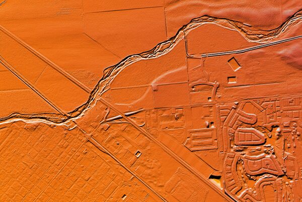
The provided DEM via GMG format was too coarse for hydraulic modeling as key hydraulic features (such as levee crests) were not adequately represented. The first step was therefore to process the 20Gb of LiDAR data into a higher resolution DEM. A 10ft DEM was created, a small part of which is illustrated below.
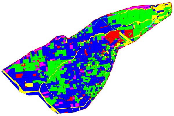
Cross-sections were extracted from the 10ft DEM, with Manning’s n values extracted from the provided GIS land use layer shown in the image below.
The Manning’s n values adopted were as provided and are tabulated below with comments on their applicability.
| Apparent Land Use | Manning's n | Colour (in image above) | Comment |
|---|---|---|---|
| Urban Areas | 0.04 | Red | Acceptable value when representing the combination of roads (0.02) and buildings, gardens and fences (0.08 to 0.30), especially if the roads are wide. |
| Cropping/Cultivation | 0.10 | Green | Representative of established medium density crops. |
| Cropping/Cultivation | 0.12 | Blue | Representative of established medium to high density crops. |
| Cropping/Cultivation | 0.15 | Magenta | Representative of established high density crops. |
| Creek | 0.20 | Yellow | Would consider this value very high. A quick inspection of the creek photos taken near structures would indicate that maybe in the upper reaches where there seems to be reasonably dense vegetation in the creek that this value is representative, but even so we still consider this value to be high in this case. In the lower reaches the creek seems quite open with little vegetation (more representative of an n value from 0.04 to 0.08). |
| Creek | 0.25 | Cyan | See comment above. |
To check these Manning's 'n' assumptions, a sensitivity testing was completed on the in-bank roughness and is detailed further in the following sections.
Boundary Conditions
Open Boundaries
A single hydrograph, derived from a previous hydrologic analysis was applied as a QT boundary via a 1d_bc. All outflow from the model was assumed to be only via the main channel (i.e. there was no water level boundary applied to the 2D overbank domain).
1D/2D Linking
The 1D river channel model was linked to the 2D model using HX cells along the top of either natural or build levees on either side of the channel. These locations defined the location of spill into the floodplain and are the key control on how much flow can interact between the floodplain and river conveyance area. The elevations along these levees were extracted from the 10ft DEM, and other significant features were included in the TUFLOW model as 3D GIS breakline layers, ensuring the hydraulic control is represented in the grid regardless of cell size.
Results - No Infiltration
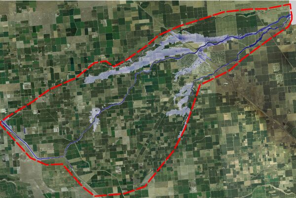
The flood extent from the 100ft 2D grid model with no infiltration and Manning's 'n' within the channel of 0.2 is shown below.
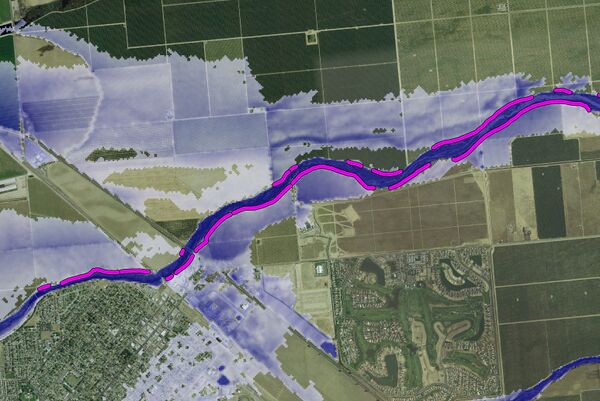
Levee Overtopping Assessment
To assess the timing and location of where levee banks were overtopped, the TGC was setup with the evacuation route command:
Read GIS Z Shape Route == shp\2d_zshr_T3_levees_001_L.shp | shp\2d_zsh_T3_levees_001_P.shp.
Via review of the RC Map Output Data Type and the _RCP output point layer we can identify sections of the levee where a breach has occured (refer below).
Sensitivity Creek Manning's n Test (Scenario 100ft n0.1)
As discussed in the Manning’s n table above, the main creek n value of 0.20 is considered very high, especially in the lower reaches of the study area. A sensitivity analysis was carried out by lowering all the Manning’s n values in the main channel (modelled as 1D cross-sections) to 0.10.
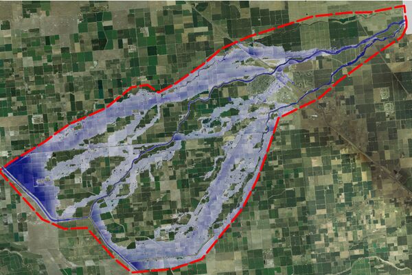
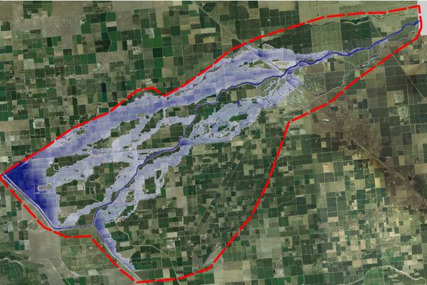
The image below shows the flood depths and extent for the two non-infiltration simulations at 100ft resolution (left with channel 'n' = 0.2, right with channel 'n' = 0.1). Some significant deviations in flood extent can be observed, particularly south of the main channel. This can be largely attributed to the higher conveyance in the channel for the 'n'=0.1 case.
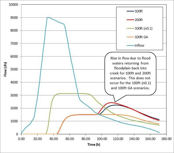
The effect of channel roughness can also be seen in hydrograph outflows from the model downstream boundary (refer figure below).
Of particular interest is that reducing the n value to 0.1 has a significant effect on the arrival time of the flood waters at the model outlet (much earlier), and reduces the volume of water flowing onto the floodplain by around 20% due to the higher conveyance of the creek. Also of interest is that for the n=0.2 scenario, some overbank floodwaters return to the main creek near the model outlet causing a delayed second rise in the outlet flow hydrographs as illustrated in the chart further below. This effect does not occur for the n=0.1 scenario, with all overbank floodwaters remaining on the floodplain.
Please note the scenarios provided in the legend below are as follows:
- 100ft = 100ft cell resolution, no infiltration and channel roughness of 'n' = 0.2
- 200ft = 200ft cell resolution, no infiltration and channel roughness of 'n' = 0.2
- 100ft (n0.1) = 100ft cell resolution, no infiltration and channel roughness of 'n' = 0.1
- 100ft GA = 100ft cell resolution, Green and Ampt infiltration with channel roughness of 'n' = 0.2
- Inflow = Hydrograph input at northeastern QT boundary.
Green and Ampt Infiltration Setup
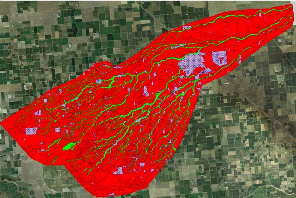
Provided soils layers were roughly classified into two soil types for the purposes of demonstrating the Green-Ampt infiltration feature in TUFLOW. The soils are shown in the image below where:
- Red indicates a Sandy Loam.
- Green is Sand.
- The blue cross-hatched areas are the Urban land use zones modeled in Challenge 3. These areas were assigned a 90% impervious parameter that restricts the rate of water entering the underlying soils. The Green-Ampt parameters used were the USDR soil type classifications which are built into TUFLOW’s internal soils database. The parameters for the two soils are tabulated below.
| USDR Soil Type | Suction (inches) | Hydraulic Conductivity (inches/h) | Porosity (fraction) |
|---|---|---|---|
| Sandy Loam | 4.3 | 0.43 | 0.412 |
| Sand | 1.95 | 4.6 | 0.417 |
The underlying soil was assumed to have an infinite depth to saturation (saturation depths/levels can be specified as 3D surfaces in TUFLOW if known). The soils were also set to have an initial moisture content of zero.
The 100ft and 200ft simulations were re-run with Green-Ampt infiltration switched on. The resulting peak flood depths map for the 100ft simulation is shown in the image below (right) whilst the 100ft without infiltration is provided on the right. As can be seen, the extent of inundation is significantly reduced with floodwaters infiltrating before reaching the model extents or returning to the main channel.
The mass balance reporting from TUFLOW indicates over half (58%) of the water infiltrates into the ground during the 171 hour simulation. This reduction in volume can also be observed via the “100ft GA” flow hydrograph show above.
Conclusion
In this challenge, we explored typical non-urban stream of the California Central Valley, with scenarios of various infiltration and flood levees adopted. From this, we gained a better understanding of the influence of flood levees on surface water behaviour, understanding of the Green Ampt infiltration method and USDR soil types, and a better understanding of nested 1D/2D models.
Congratulations on finishing the FMA Demo Model 3. Please click here to return the Wiki Main Page.
