TUFLOW Remapping

Introduction

With the release of TUFLOW 2020, the combination of Quadtree mesh and Sub-grid Sampling (SGS) method has offered great flexibility to build a model with a range of mesh sizes. SGS samples the digital elevation model (DEM) at a number of points within a cell and computing the water surface elevation as a function of cell stored volume. With SGS, cells and faces can be considered as "partially wet", and this means the impact of the sub-grid scale geometry can be represented by cells with larger sizes. The example below shows a Quadtree model with 10/20m cell size can conduct water as smoothly as a 2.5/5/10/20m model along a narrow stream.

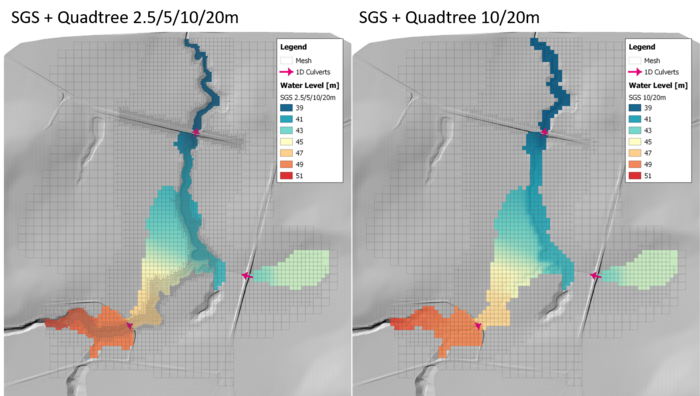
Figure 1 Water level simulation results with SGS. Left: 2.5/5/10/20m Quadtree model. Right: 10/20m Quadtree model.

On the other hand, the same model running without SGS method creates notably different results in the distance of water travelled and the area of inundation on floodplain due to the poor geometry representation.

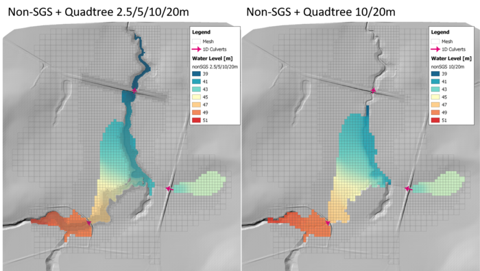
Figure 2 Water level simulation results without SGS. Left: 2.5/5/10/20m Quadtree model. Right: 10/20m Quadtree model.

These examples indicate the mesh size sensitivities of a SGS model are significantly reduced, and thus modellers are increasingly using coarser mesh at areas far away from the location of interest. However, this has also create a challenge for how to output water depth at those coarser cells. The example below shows even the 10/20m mesh and the 2.5/5/10/20m mesh models produce similar water level, but the depth map output is much 'smoother'in the model with finer meshes.

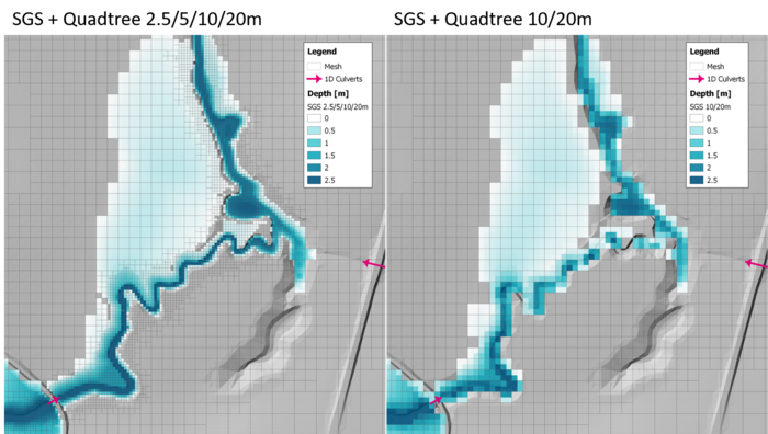
Figure 3 Water depth simulation results with SGS. Left: 2.5/5/10/20m Quadtree model. Right: 10/20m Quadtree model.

In TUFLOW, the depth output is interpolated from the depths at nearest cell centre and cell corners surrounding the output grid. The interpolated depth may not perfectly represent the actual depth, since TUFLOW doesn't store the under laying high resolution DEM values at the moment.

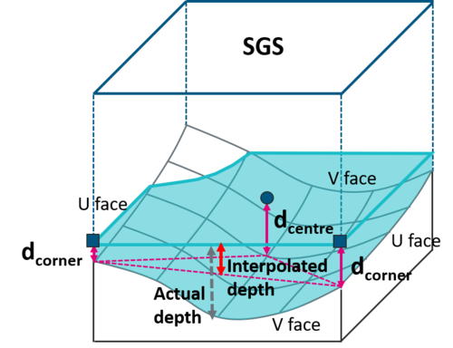
Figure 4 TIN interpolation used for water depth map output with SGS.

While we are developing high resolution SGS output in the future release to address this issue, we have also added a new functionality in the ASC_to_ASC utility to 'remap' a water level grid to a finer DEM grid. This page introduce how to use the ASC_to_ASC remap function, and also discuss the limitation of the method.

Remap Water Level to Finer DEM

The remap function in the ASC_to_ASC remaps a water level grid to a high resolution DEM using TIN interpolation. It outputs a high resolution water level grid and a high resolution depth grid.

asc_to_asc.exe -remap -wl lowres_h.asc -dem DEM_highres.asc

In this command:
"-wl <wl_file>"
Sets the coarser resolution water level grid to remap from.
"-dem <dem_file>"
Sets the finer resolution DEM.
The figure below overlays the remapped water depth on top of the 10/20m model water level output, and compared it to the original water depth output. As can be seen, smooth water depth along the gully and flood fringes is produced by the post process utility.

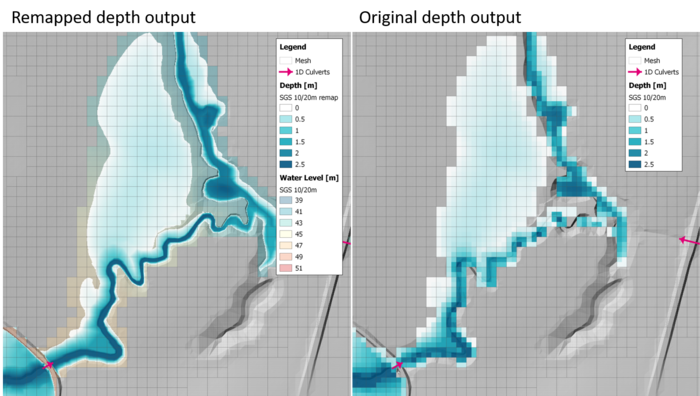
Figure 5 Remapped vs original water depth for 10/20m mesh SGS model.

The next example presents the water level output and the remapped depth output in a river flood modelling. As can be seen, large portions of small buildings are submerged by water level output due to the relative size of the mesh and the buildings. However, remapped depth shows smooth fringes around the buildings.

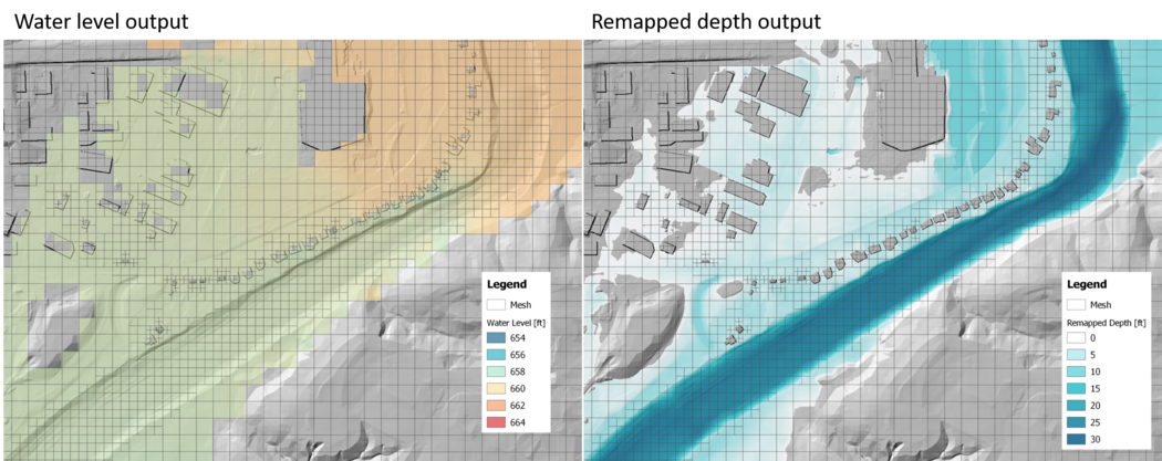
Figure 6 Water level output and remapped water depth in a river flood model.

Remap Other Output Grids

The utility can also remap extra grid files (e.g. a hazard output) to the resolution of the DEM file.

asc_to_asc.exe -remap -wl lowres_h.asc -dem DEM_highres.asc lowers_hazard.asc

This command reads in an extra grid 'lowers_hazard.asc' and remaps it to the finder DEM resolution.The figure below compares the original hazard output from the 10/20m SGS model and the remapped hazard output.

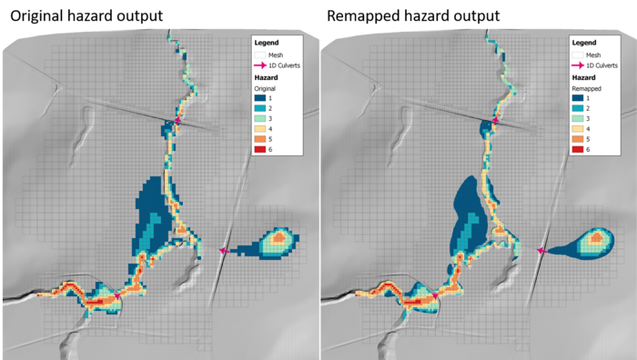
Figure 7 Remapped vs original hazard output for 10/20m mesh SGS model.

It is important to note that, for output types other than depth, this utility does NOT interpolate the result from the coarser grid to the finer grid, but only extended/reduced the output extent to the dry/wet extent. Therefore, the resolution of the remapped hazard above remains the same as the original output grid. The interpolation is not conducted for the following reasons:

• Hazard categories are usually depended on both water depth and velocity, and it is not straight forward to interpolate a cell averaged velocity to sub-cell scale with varying water depth.
• Even if this can be done based on empirical relationship between depth and velocity, the obtained velocity is much less reliable than a actual output from a model with finer mesh.

Therefore, we highly recommend refining the mesh size directly a the location where user wants to obtain finer velocity or hazard output. The figure below shows the hazard output from the 2.5/5/10/20m model, and as can be seen the result is much smoother along the gully.

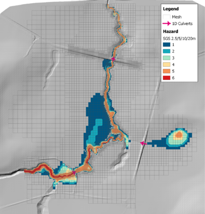
Figure 8 Original hazard output for 2.5/5/10/20m mesh SGS model.

1D/2D SX Links Defined Using 1D Nodes (1d_nwk)

As of the 2017 release of TUFLOW, nodes within a 1d_nwk file can be used to specify the location of 1D/2D boundary cells and also automatically assign an estimate of the appropriate number of 2D cells for the connection.

For a culvert, this is done by snapping a 1d_nwk point feature to the end of the 1d_nwk line feature and setting the 1d_nwk point attributes:

• Type = Node
• UCS = T
• CONN_1D_2D = SX

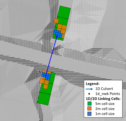
2D cells will be automatically selected as a 1D/2D SX links. The number of cells that are associated with the 1D/2D SX link will be defined by the nodal storage of the 1D channel. The figure below shows the 1D/2D linking cells in the 5m, 2m and 1m cell size models using this method.

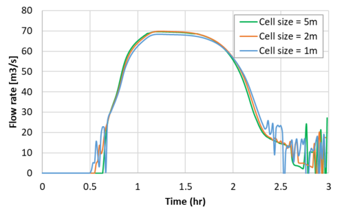
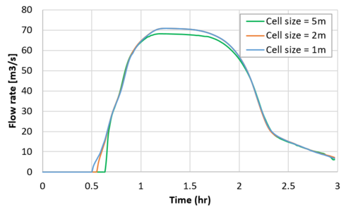
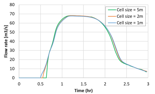
The modelled flow rates are shown in the figure below. As can be seen, comparable peak flow rates are obtained regardless of the cell size (i.e. cell size convergence is demonstrated). The stability in the 1m cell size case has been improved markedly, though there are still some oscillations at low flows.

SX Boundary Lines (2d_bc)

2d_bc SX line features are often used to connect 1D structure to the 2D domain if the structure width is greater than one 2D cell wide (e.g. Tutorial Module02). This configuration not only increases the number of 1D/2D linking cells, it also has the added benefit of defining the 1D/2D boundary cells at the approximate location of the inlet/outlet of the 1D culvert. An additional benefit of this approach is that the "width" of the linking cells remains similar in length and location irrespective of 2D cell size.

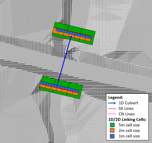
The 1D/2D linking cells in the 5m, 2m and 1m cell size models are shown in the the figure below.

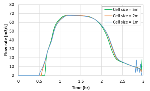
The result below indicates cell size convergence is achieved, the flow oscillations have also been reduced (compared to the model using the 1d_nwk Node 1D/2D link method).

SX Storage Factor (2d_bc)

A new "SX Storage Factor" feature was been added to TUFLOW in the 2017 release. As the name suggests, this feature adds additional storage to the 1D/2D linking (SX) cells. The storage factor is specified by adjusting the 2d_bc "a" attribute value. "a" is treated as a storage multiplier. For example, specifying an "a" value of 2.0 doubles the storage associated with the 1D/2D boundary. Note that an "a" value of 0.0 assumes a multiplier of 1.0.

The modelling result with an "a" value of 2.0 are presented in the figure below. The flow rate is now very smooth and the difference in peak flow rates is negligible.

Testing has shown small increases in storage usually has immeasurable effect on results, however, sensitivity testing is recommended to confirm this assumption in different models. For example, if specifying an "a" value of 2 stabilises the link, sensitivity test by increasing "a" further to 3. If there is no appreciable or unacceptable change in results, increasing the storage by a factor within these bounds can be considered to have negligible effect on results.

SX Boundary Regions/Polygons (2d_bc)

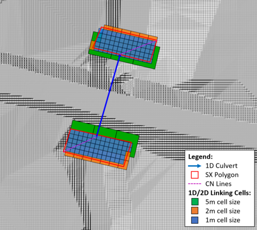
SX boundary regions/polygons are another feature that was added for the 2017 TUFLOW release. Polygons can now be used as a 2d_bc SX input. All cells with a cell centre within the polygon are set as SX cells. A CN line is required to connect the 1D feature to the SX polygon, snapped to any vertex on the perimeter of the polygon. An example of this configuration and the 1D/2D linking cells produced in the 5m, 2m and 1m cell size models are shown in the figure below.

The modelling results are presented in the figure below. Again, cell size convergence is demonstrated and the oscillations at low flow is removed.

Conclusion

When the spatial resolution of a model is increased (i.e. cell size reduced) review of result sensitivity at 1D/2D SX link locations is recommended. This can be done quickly and easily by plotting 1D results and checking for unwanted oscillations. This page demonstrated some useful methods for stabilising 1D/2D boundary (SX) links, in particular where the 1D structure is large in comparison to the 2D cell size. Available options that were introduced included reviewing the 1D timestep, using 1D nodes to define the 1D/2D boundary link, SX boundary lines, SX storage factors and SX boundary polygons.