SMS Tips: Difference between revisions
| Line 11: | Line 11: | ||
Open the results, by either opening the .2dm and the results files or by opening the .sup file. |
Open the results, by either opening the .2dm and the results files or by opening the .sup file. |
||
==Scalar Data== |
==Scalar Data== |
||
Once you have results loaded into SMS, open the Display Options Dialogue, in the menu items select ''Display >> Display Options...''.<br> |
|||
'''TIP:''' The shortcut key to bring up the Display Options dialogue is Control + D. |
|||
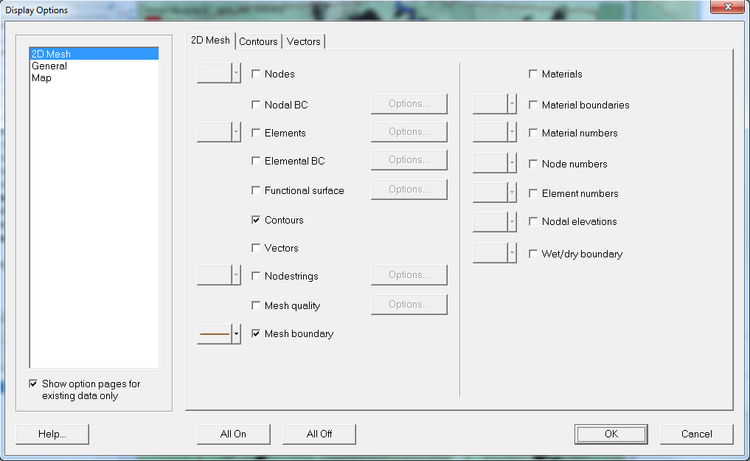
In the Display Options dialogue, ensure that you are in the 2D Mesh module in the pane to the left. In the 2D mesh tab, you get a list of options ticking the check box will make an item visible. To see just the scalar results, turn everything off, except '''Contours'''.<br> |
|||
<br> |
|||
[[File:SMS 10p1 Display Options.png|750px|SMS 10.1 Display Options]]<br> |
|||
[[File:SMS 10p1 M01 Results Available.png|300px|right|frame]] |
|||
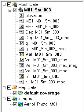
In the project window under Mesh Data is a list of the scalar and vector datasets available.<br> |
|||
Scalar datasets are indicated by the icon '''123''' and vector datasets have 2 arrows as the icon. In the image is the full list of datasets for the TUFLOW tutorial model (Module 1).<br> |
|||
A number of datasets appear twice, for example Vel M01_5m_003 is available for viewing as a scalar dataset or a vector dataset (see next section). |
|||
An '''_max''' in the dataset name indicates that this in maximums throughout the simulation. '''Dep M01_5m_003''' contains the time varying data and '''Dep M01_5m_003_max''' contains the peak depths. |
|||
*Select the scalar dataset that you wish to view.<br> |
|||
*In the "'''Time Steps'''" window, select a timestep and use the up and down arrows to step through the results. |
|||
=== Contouring Options === |
|||
There are numerous options for controlling how the scalar results display (colour profile, contour increment, transparency). This is controlled in the ''Contour'' tab in the Display Options dialogue. A brief guide is given below, users are encouraged to experiment. |
|||
*Bring up the Display Options dialogue, and select the "Contour" tab under 2D Mesh. |
|||
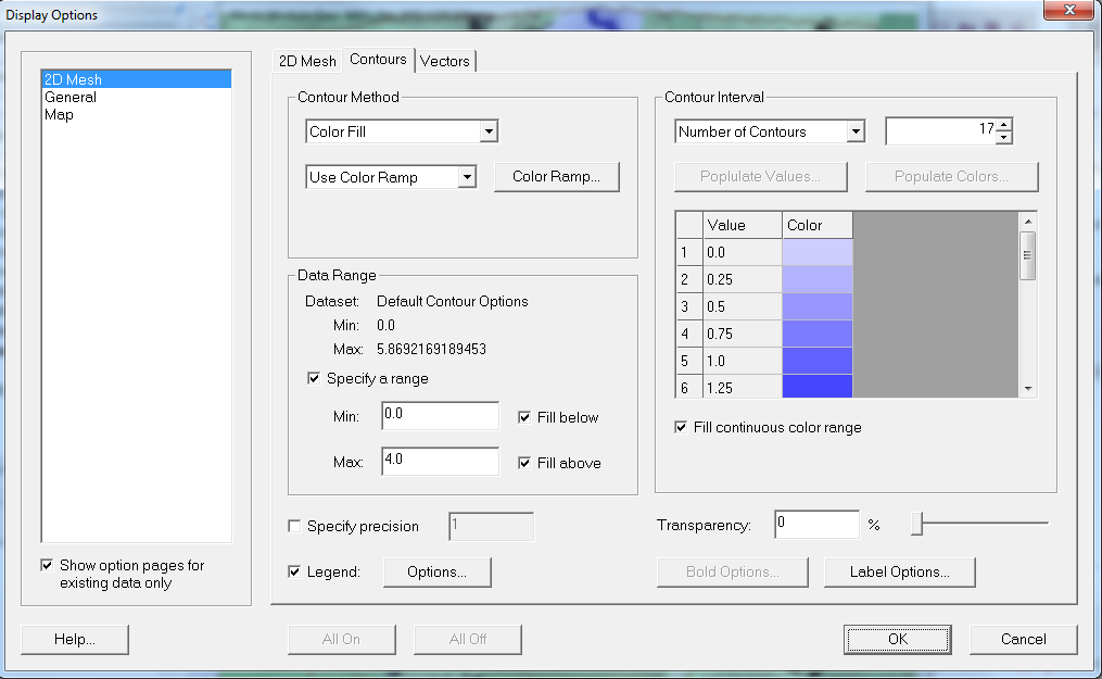
*Under ''Contour Method'' select '''Color Fill'''.<br> |
|||
'''TIP:'''''Normal Linear'' can be used to display contour lines only, and ''Color and Linear'' displays both contour shading and contour lines.<br> |
|||
[[File:SMS 10p1 Scalar Results Contouring.png|frame|none]] |
|||
<br> |
|||
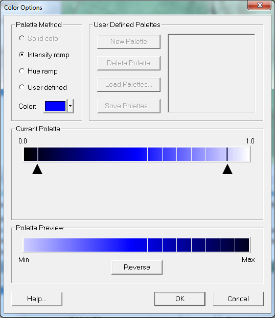
Under "Color Ramp" you can choose the colour profile. There are numerous options here, feel free to experiment. I have chosen an ''Intensity Ramp'' varying from light blue to dark blue.<br> |
|||
[[File:SMS 10p1 Colour Ramp.png|frame|none]] |
|||
<br> |
|||
In the ''Data Range'' section of the Display Options dialogue there is a summary of the minimum and maximum data values for the selected dataset. A range can specified here, by checking the "''Specify a range''" option. In the image below an upper range of 4.0 metres, anything above this depth will display in the upper contour range (dark blue).<br> |
|||
'''TIP:''' by specifying a range and un-checking "Fill Above" or "Fill Below" you can restrict the display range. For example, setting a minimum of 0.1m and un-checking "Fill Below" any depths less than 0.1m will not be displayed. |
|||
A transparency can also be set in this dialogue, this can be used to make aerial photos visible beneath the contouring. |
|||
==Vectors== |
==Vectors== |
||
==Animations== |
==Animations== |
||
Revision as of 13:51, 27 September 2011
Introduction
This page contains a brief introduction to the SMS software, for more information please see the SMS wiki or the AQUAVEO Forums.
Viewing Results
To view results in SMS we need at least two files open. The first is the TUFLOW mesh, this contains information on the location, cells and elevations within the model. The 2D mesh is created by TUFLOW and is outputted with the .2dm extension. A mesh is created for every TUFLOW simulation and has the same name as the TUFLOW simulation. For example if the simulation control file is named M01_5m_003.tcf the TUFLOW mesh will be a file called M01_5m_003.2dm.
Once the mesh has been loaded, the TUFLOW results can be loaded. TUFLOW results can outputted in either the .dat format (1 results file format per output type) or in recent versions of TUFLOW the .xmdf (one output file that contains all of the results).
TUFLOW also writes out a .sup file which contains instructions for SMS to open the 2D mesh first and then the TUFLOW results.
Open the results, by either opening the .2dm and the results files or by opening the .sup file.
Scalar Data
Once you have results loaded into SMS, open the Display Options Dialogue, in the menu items select Display >> Display Options....
TIP: The shortcut key to bring up the Display Options dialogue is Control + D.
In the Display Options dialogue, ensure that you are in the 2D Mesh module in the pane to the left. In the 2D mesh tab, you get a list of options ticking the check box will make an item visible. To see just the scalar results, turn everything off, except Contours.


In the project window under Mesh Data is a list of the scalar and vector datasets available.
Scalar datasets are indicated by the icon 123 and vector datasets have 2 arrows as the icon. In the image is the full list of datasets for the TUFLOW tutorial model (Module 1).
A number of datasets appear twice, for example Vel M01_5m_003 is available for viewing as a scalar dataset or a vector dataset (see next section).
An _max in the dataset name indicates that this in maximums throughout the simulation. Dep M01_5m_003 contains the time varying data and Dep M01_5m_003_max contains the peak depths.
- Select the scalar dataset that you wish to view.
- In the "Time Steps" window, select a timestep and use the up and down arrows to step through the results.
Contouring Options
There are numerous options for controlling how the scalar results display (colour profile, contour increment, transparency). This is controlled in the Contour tab in the Display Options dialogue. A brief guide is given below, users are encouraged to experiment.
- Bring up the Display Options dialogue, and select the "Contour" tab under 2D Mesh.
- Under Contour Method select Color Fill.
TIP:Normal Linear can be used to display contour lines only, and Color and Linear displays both contour shading and contour lines.

Under "Color Ramp" you can choose the colour profile. There are numerous options here, feel free to experiment. I have chosen an Intensity Ramp varying from light blue to dark blue.

In the Data Range section of the Display Options dialogue there is a summary of the minimum and maximum data values for the selected dataset. A range can specified here, by checking the "Specify a range" option. In the image below an upper range of 4.0 metres, anything above this depth will display in the upper contour range (dark blue).
TIP: by specifying a range and un-checking "Fill Above" or "Fill Below" you can restrict the display range. For example, setting a minimum of 0.1m and un-checking "Fill Below" any depths less than 0.1m will not be displayed.
A transparency can also be set in this dialogue, this can be used to make aerial photos visible beneath the contouring.