TUFLOW 1D2D SX Advice

Introduction

With the release of TUFLOW HPC (in 2017) and the continuous improvement of GPU hardware compute capability, there is an industry trend for models of higher resolution. As such, the 2D cell size in flood models is becoming smaller and smaller. Testing has shown in some instances reducing the 2D cell size may cause increase model instability at 1D/2D SX locations. This Wiki page discusses this observation, the cause and available methods to correct the instability. Topics of discussion include:

• 1D timestep selection
  
• Use of a 1D Node to assign 1D/2D boundary condition cells
  
• Use of SX 1D/2D boundary condition lines
  
• Application of a SX Storage Factor
  
• Use of SX 1D/2D boundary condition polygons
  

These methods can be applied to both TUFLOW Classic and HPC using the 2017 release or newer. For the purpose of this demonstration TUFLOW HPC has been used.

Base Case

A simple 1D/2D model has been constructed based on Tutorial Module 2. SX points have been used to connect a 1D culvert (FC01.2) with the 2D domain. The culvert details are:

• Type = R (Rectangular)
• Number of barrels = 5
• Width per culvert = 2.4m (i.e the total width of the bank of culverts is 12m)
• Height = 1.2m

Three 2D cell resolutions have been tested: 5m, 2m and 1m. The figure below shows the 1D/2D linking cells of the culvert.

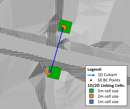
This figure highlights the variation in 2D storage volume associated with the 1D/2D SX connections. The storage associated with a single 1D/2D linking cell for each cell size is:

• 5m 2D cell size = 25m²/m
• 2m 2D cell size = 4m²/m
• 1m 2D cell size = 1m²/m
  

The modelled flow rates in the culvert is presented in the figure below.

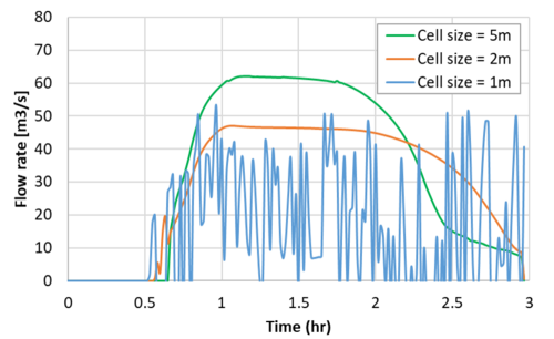
Two key observations can be made:

• The 1D/2D link associated with the 1m 2D cell size is not stable.
• The flow rate results through the 1D culvert decrease with cell size. This is an issue. It indicates cell size convergence (i.e. consistent results independent of cell size) was not achieved. This is caused by the 2D storage volume associated with the 1D/2D connection being insufficient compared to the flow area associated with the 1D channel (12m width). As a result, the 2D boundary cell is the model feature limiting flow exchange between the 1D and 2D, rather than the dimension and hydraulics associated with the 1D structure.

1D Timestep

Selection of a 1D timestep that is too large can cause instability. The TUFLOW manual includes some discussion on 1D timestep selection and courant number criterion. Conceptually a 1D timestep should be chosen to ensure a volume of water does not travel a distance longer than the shortest 1D channel within a model. For example, if the flow velocity and celerity is 5m/s and the 1D channel length is 10 metres, the 1D timestep should be less than 2 seconds. To provide some tolerance for faster flows associated with different flood events, a timestep of 1 second may be appropriate.

During real world studies it is good practice to check the 1D timestep sensitivity.

• Select a 1D timestep based on the smallest channel length and the expected flow velocity within your model.
  
• Trial using a smaller 1D timestep to establish whether the problem is timestep related.
  

If the instability is not timestep related, reducing the timestep should have a negligible change in results.

A 1s 1D timestep has been used for this testing. It is appropriate for the 1D features being modelled.

Note: The 1D timestep for a HPC 1D/2D linked model is the 'limiting' timestep the 1D solver can use. The 1D solver has been reconfigured to act as an adaptive/varying timestep solution, and the 1D timesteps are set at different multiple of 2D timesteps.

Use 1D Nodes to create 1D/2D links

As of the 2017 release of TUFLOW, nodes within a 1d_nwk file can be used to specify the location of 1D/2D boundary cells and also automatically assign an estimate of the appropriate number of 2D cells for the connection.

For a culvert, this is done by snapping a 1d_nwk point feature to the end of the 1d_nwk line feature and setting the 1d_nwk point attributes.

• Type = Node
• UCS = T
• CONN_1D_2D = SX

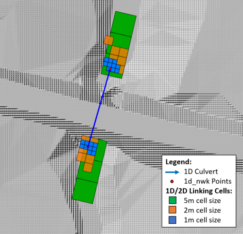
2D cells will be automatically selected as a 1D/2D SX links. The number of cells that are associated with the 1D/2D SX link will be defined by the nodal storage of the 1D channel. The figure below shows the 1D/2D linking cells in the 5m, 2m and 1m cell size models using this method.

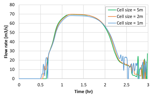
The modelled flow rates are shown in the figure below. As can be seen, comparable peak flow rates are obtained regardless of the cell size (i.e. cell size convergence is demonstrated). The stability in the 1m cell size case has been improved markedly, though there are still some oscillations at low flows.

SX Boundary Lines

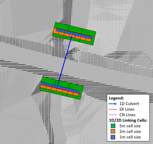
2d_bc SX line features are often used to connect 1D structure to the 2D domain if the structure width is greater than one 2D cell wide (e.g. Tutorial Module02). This configuration not only increases the number of 1D/2D linking cells, it also has the added benefit of defining the 1D/2D boundary cells at the approximate location of the inlet/outlet of the 1D culvert. An additional benefit of this approach is that the "width" of the linking cells remains similar in length and location irrespective of 2D cell size.

The 1D/2D linking cells in the 5m, 2m and 1m cell size models are shown in the the figure below.

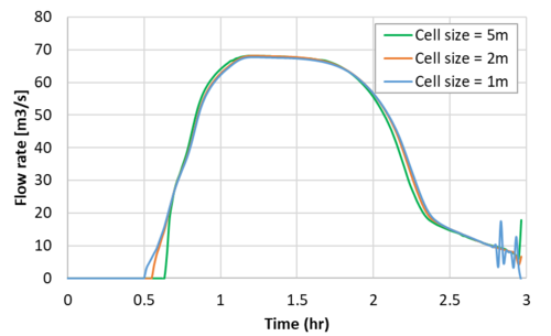
The result below indicates cell size convergence is achieved, the flow oscillations have also been reduced (compared to the model using the 1d_nwk Node 1D/2D link method).

SX Storage Factor

A new "SX Storage Factor" feature was been added to TUFLOW in the 2017 release. As the name suggests, this feature adds additional storage to the 1D/2D linking (SX) cells. The storage factor is specified by adjusting the 2d_bc "a" attribute value. "a" is treated as a storage multiplier. For example, specifying an "a" value of 2.0 doubles the storage associated with the 1D/2D boundary. Note that an "a" value of 0.0 assumes a multiplier of 1.0.

The modelling result with an "a" value of 2.0 are presented in the figure below. The flow rate is now very smooth and the difference in peak flow rates is negligible.

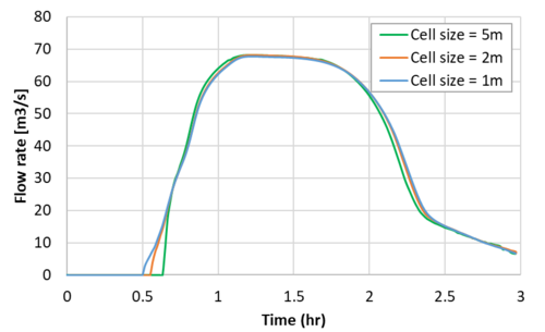
Testing has shown small increases in storage usually has immeasurable effect on results, however, sensitivity testing is recommended to confirm this assumption in different models. For example, if specifying an "a" value of 2 stabilises the link, sensitivity test by increasing "a" further to 3. If there is no appreciable or unacceptable change in results, increasing the storage by a factor within these bounds can be considered to have negligible effect on results.

SX Boundary Regions/Polygons

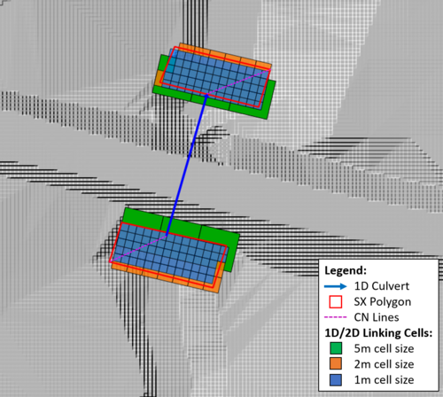
SX boundary regions/polygons are another feature that was added for the 2017 TUFLOW release. Polygons can now be used as a 2d_bc SX input. All cells with a cell centre within the polygon are set as SX cells. A CN line is required to connect the 1D feature to the SX polygon, snapped to any vertex on the perimeter of the polygon. An example of this configuration and the 1D/2D linking cells produced in the 5m, 2m and 1m cell size models are shown in the figure below.

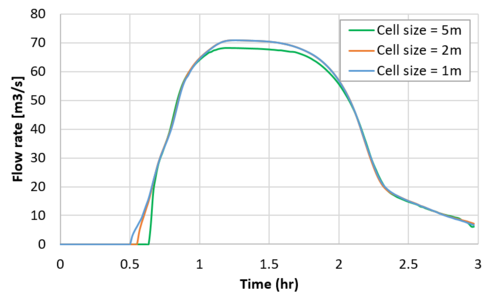
The modelling results are presented in the figure below. Again, cell size convergence is demonstrated and the oscillations at low flow is removed.

Conclusion

When the spatial resolution of a model is increased (i.e. cell size reduced) review of result sensitivity at 1D/2D SX link locations is recommended. This can be done quickly and easily by plotting 1D results and checking for unwanted oscillations. This page demonstrated some useful methods for stabilising 1D/2D boundary (SX) links, in particular where the 1D structure is large in comparison to the 2D cell size. Available options that were introduced included reviewing the 1D timestep, using 1D nodes to define the 1D/2D boundary link, SX boundary lines, SX storage factors and SX boundary polygons.