View Results in QGIS with the TUFLOW Viewer Archive
Introduction
The QGIS TUFLOW Viewer replaces Crayfish and TUPLOT as the TUFLOW result viewer for QGIS for version 3.6 onwards. It allows for much larger datasets to be viewed and analysed more efficiently than before. It uses the Mesh Data Abstraction Library (MDAL) available in QGIS to display and interact with TUFLOW map output results, and the TUFLOW results python library (the same library used by TUPLOT in earlier versions of QGIS) for viewing TUFLOW time series results.
Installation
- Ensure that QGIS 3.20 or later is installed.
- Open QGIS.
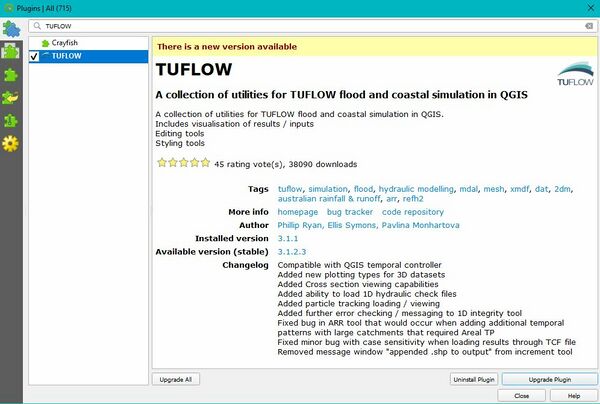
- Install the TUFLOW Viewer by selecting Plugins >> Manage and Install Plugins >> TUFLOW from the plugin directory.

This will now show the TUFLOW Viewer Toolbar, click on the symbol below to open the Viewer within your mapping window:

Method
The results can either be loaded in via File Load Results or Right Click in the Open Results panel and choose Load Results. Load results uses a TCF, TLF or FVC and will load in all results (Map Outputs and Time Series). Alternatively, you can open the Map Outputs and Time Series results independently using:
- Load Results - Map Outputs --> Select map output mesh results file (*.xmdf, *.dat, *.2dm, *.xmdf.sup, *.dat.sup)
- Load Results - Time Series --> Select time series output results (*.tpc)
- From Load Results, navigate to the TUFLOW\runs Folder and add the M01_5m_002.tcf file. Although this is the control file, as mentioned above this will use the paths within it to load all results.
- Selecting the control file will load all the specified XMDF outputs, in the later tutorials where 1D ESTRY components are added this will also load in the 1D time series results.
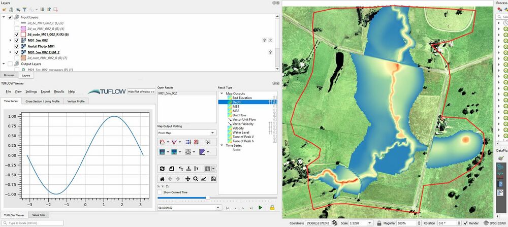
- Select "M01_5m_002" from the Open Results list and then select Depth. Scroll through the output times. The results should update as new output times are selected. The window should look similar to the below image:
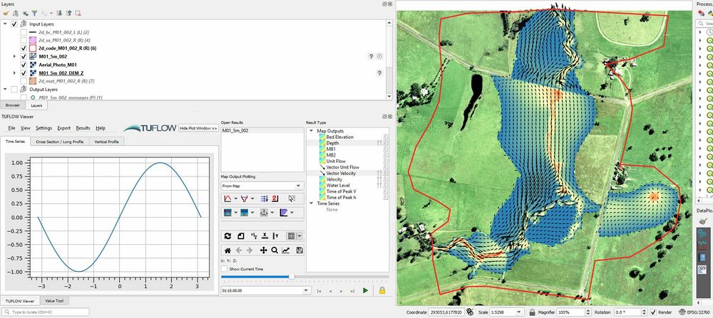
- Both the depth and water level (head) are scalar results. Using the Viewer both depth scalar results and velocity vector results can be visualised at the same time. The vector output shows both direction and magnitude. The "Display Contour" and "Display Vectors" options should now be selectable. Scrolling through the output times should display both shading (velocity magnitude) and arrows (direction).
- Both the depth and water level (head) are scalar results. Using the Viewer both depth scalar results and velocity vector results can be visualised at the same time. The vector output shows both direction and magnitude. The "Display Contour" and "Display Vectors" options should now be selectable. Scrolling through the output times should display both shading (velocity magnitude) and arrows (direction).
- The appearance of the contour and vectors can be changed. Right click on Vector velocity and select Properties. Tick the "Display on User Grid" option to 'have an XY spacing of 10 px. Select apply to update the display.
- Please feel free to experiment with the visualisation options and get a feel for your TUFLOW results. Do the results look sensible? What happens at the road crossings?
- Please feel free to experiment with the visualisation options and get a feel for your TUFLOW results. Do the results look sensible? What happens at the road crossings?


- Tip The following page here, shows the wide range of other options available in the TUFLOW Viewer, its an extremely powerful tool for any modeller!
Conclusion
We have covered the basics of viewing 2D TUFLOW results in QGIS using the TUFLOW Viewer Plugin. Please return to the tutorial model, Module 1. In the next step we review the performance of the TUFLOW model (warnings, checks and mass balance), to return please click here
