1D Manholes

Page Under Construction

Introduction

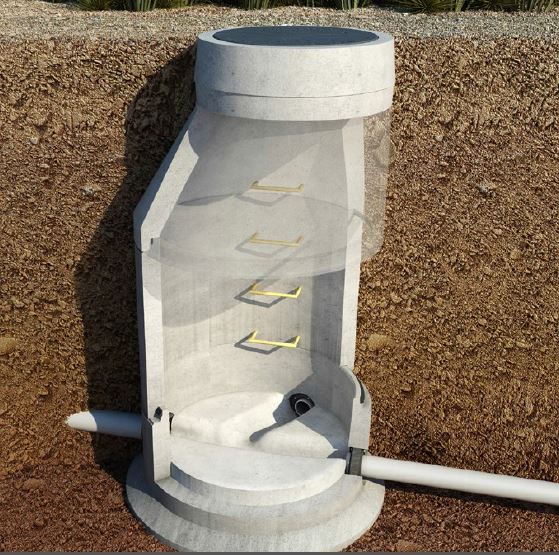
Manholes are typically chambers used to provide one or all of the following; maintenance access, change in culvert direction, connections and change in culvert dimensions. By default, manholes are automatically created within TUFLOW at all culvert nodes, any manually created manhole will override the automatically created manhole.

Manholes are used at culvert junctions to dissipate energy due to:

• Expansion/contraction of flow within the manhole chamber and outlet culverts.
• Change in direction of the culverts (i.e. a bend/deflection).
• Change in height, width or diameter and/or invert level of the adjoining culverts.

The presence of a manhole at a junction point will override the exit loss of any culvert discharging into the manhole and entrance loss of any culvert taking from our of the manhole.

There are 3 types of manholes:

• "C" for circular chambers.
• "R" for rectangular chambers.
• "J" for junctions without a chamber

Losses

When modelling conduit pipe flows, the head losses that the flow in pipe are subject to are made up of major losses (or friction losses) and minor losses (or local losses). Major losses are caused by forces between the flow and wetted perimeter of the conduit. Minor losses are caused by disruption to the flow due to bends, cross-sectional changes, fittings such as manholes and steps in the bed profile. Major losses are represented through the specification of a friction coefficient. The representation of minor losses, particularly or gravity networks, is at manholes and requires separate treatment. The default TUFLOW/Estry manhole loss approach uses the Engelund method explained in section 5.12.5.4 of the TUFLOW user manual. The Engelund approach provides an automatic method for determining the loss coefficients as presented below. Of note is that the coefficients are recalculated every timestep, and therefore vary depending on the flow distribution between inlet and outlet conduits and the depth of water within the manhole. The losses represented are as follows:

K_entry covers the expansion of flow within the manhole at the outlet of an inlet conduit. The coefficient is applied as the exit loss of the inlet conduit.

K_Ɵ represents the losses due to a change in direction (i.e. a bend) between inlet and outlet conduits. KƟ is determined automatically by TUFLOW based on the angle of the digitised lines of the conduits. For the inlet conduit the last two vertices of the line are used and for the outlet conduit the first two vertices.

K_drop is the loss coefficient due to a change in invert level and conduit height between inlet and outlet conduits.

K_Ɵ and K_drop are added and applied as an energy loss for each outlet conduit.

K_exit covers the contraction from the manhole and re-expansion of flow within the entrance of an outlet conduit. It is applied as an entrance loss of the outlet.

K_m is the user-defined manhole exit coefficient. The resulting headloss value is then applied, when sub-critical flow is experienced, to the standard head loss equation, i.e. dh = K*V²/2g. Where K is the loss coefficient, V is the conduit velocity and g the gravitational constant. The equations used for the Engelund loss approach are provided below:

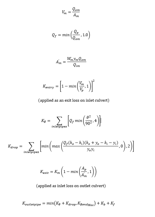
Where:
Q_p = Flow in Conduit
Q_im = Total flow into manhole
Q_om = Total flow out of manhole
y_i = Height of inlet conduit
y_o = Height of outlet conduit
h_i = Inlet conduit invert
h_o = Outlet Conduit invert
θ = Angle in degrees of inlet conduit relative to outlet conduit(θ = 0° "when the culverts are in line," θ=90° when the outlet culvert is at right angles)
Q_p = Flow in conduit outlet
W_m = Flow width in manhole (1d_mh width attribute)
y_m = Depth of water in manhole
A_m = Flow are in manhole
A'_m = Effective flow are in manhole
A_p = Flow area of conduit
K_m = Manhole Loss Parameter (1d_mh Km attribute)
K_b = Bend Loss Coefficient (1d_nwk Form_loss attribute)
K_f = Fixed Loss (1d_mh K_Fixed attribute)
K_Bendmax = Upper limit to sum of K_θ and K_drop (1d_mh K_Bend_Max attribute)

Below are three worked examples of the application of the Engelund method applied to a simple model for the following scenarios:

Single Incoming/Outgoing Pipe with no angle and no drop

Single Incoming/Outgoing Pipe with incoming bend and drop in levels

Multiple Incoming Pipes with incoming bend and drop in levels

Example 1: Single Incoming/Outgoing Pipe with No Incoming Angle or Drop

A simple TUFLOW/ESTRY model was set up as shown in Figure 1 with the parameters for the manhole and the links upstream/downstream of the manhole shown in Table 1.

Figure 1: Example Model 1 Network Schematic

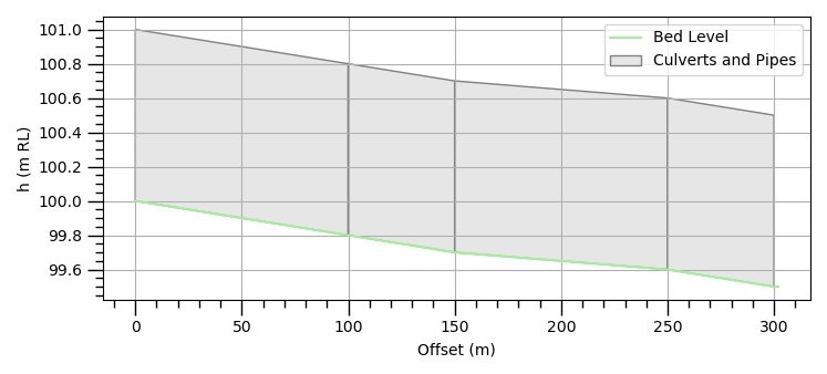
Figure 2: Example Model 1 Long Section

Parameter	Upstream Conduit	Downstream Conduit	Manhole
ID	UC-2	Manhole	DC-1
Type	R	R	R
Invert Level (m AD)	N/A	N/A	99.6
Upstream Invert Level (m AD)	99.8	99.7	N/A
Downstream Invert Level (m AD)	99.7	99.6	N/A
Width(m)	1	N/A	1
Form Loss	0	1	N/A
Flow Width(m)	N/A	N/A	1.8
K_Fixed	N/A	N/A	2
Km	N/A	N/A	1

Table 1: Relevant Model Parameters for Hand Calculations
The model was run with a steady inflow of 2m³s^-1. The resulting losses from the 1 hour steady inflow simulation are presented in the following figure.

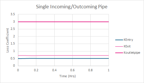
Figure 3: Example Model 1 Results-Loss Coefficients

Example 1 - Entry Losses

Entry losses are applied as an exit loss on the incoming conduit and are calculated as follows.
Where:
With other parameters defined in the section above. The calculated flow area in the manhole is 3.6m² and 1m² in the adjacent culvert whilst the flow is 2m³/s for both Q_p and Q_om. Therefore, V_m equals:
And V_p:
Using these in the K_entry equation provides a loss coefficient of:
The value matches the downstream loss coefficient for the upstream conduit shown in Figure X. The loss values are also shown in the *_TSL_P.shp file with the third value for the upstream conduit providing the entrance loss value.

Example 1 - Exit Losses

Exit losses are applied to the upstream end of the outgoing conduit and are calculated as follows:
From table 1, we can see that K_m is set to 1. A_p and A’_m are 1m² and 3.636m² respectively. Therefore, K_exit is:

Figure 3 shows that the calculated value matches those provided in the TUFLOW results. The value is also reported as the first value for the downstream conduit in the *_TSL_P.shp layer.

Example 1 - Outgoing Conduit Losses

The loss coefficient for the outgoing pipe represents the losses due to the incoming angle of the upstream conduit, any drops in inverts levels between the incoming and outgoing conduits, bend losses and any additional form losses. It is calculated as follows:

The default value of K_{Bend_max} is set to 4 but can be changed via the 1d_mh K_Bend_Max attribute. As shown above we have no angle for the incoming pipe and no drop in invert levels. Table 1 shows the K_Fixed is equal to 2 and the outgoing pipe has a form loss coefficient, to represent bend losses of 1. Therefore K_outletpipe is:

This matches the value within Figure 3 and the middle value for the downstream conduit in the *_TSL_P.shp, representing the outlet conduit losses, of 3.

Example 2: Single Incoming/Outgoing Conduit with Incoming Bend and Drop in Invert Levels

In this example, we will use the same simple setup but this time there is a 90 degree angle between the incoming and outgoing pipe as shown in the plan view in the figure below.

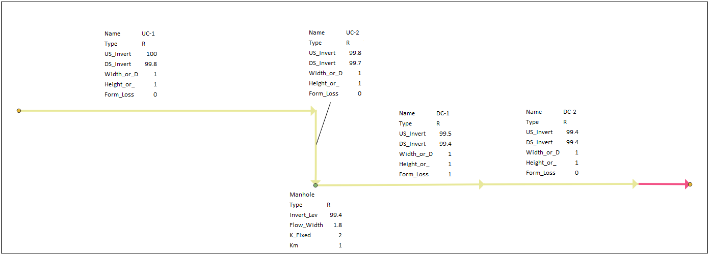
Figure 4: Example Model 2 Network Schematic

There is also a drop between the invert elevation of the incoming and outgoing conduits as shown in the difference in invert levels in table 2 below and the long profile in figure 5 . All other model parameters were kept the same including boundary inflows.

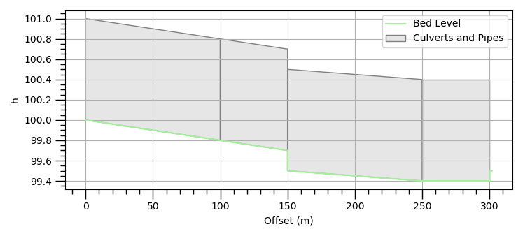
Figure 5: Example Model 2 Long Profile

The resulting simulated losses are shown in the below figure 6.

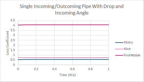
Figure 6: Example Model 2 Results-Loss Coefficients

Example 2 - Entry Losses

In this example, the flow area in the manhole is 4.12m² and 1m² in the adjacent culvert whilst the flow is 2m³/s for both Q_p and Q_om. Therefore, Vm equals:
And V_p:
From this:

Which matches the value in figure 6.

Example 2 - Exit Losses

In this example, A'_m is 4.12m², therefore K_exit:

Which matches the result in figure 6.

Example 2 - Outgoing Conduit Losses

On this occasion, we have an 90 degree angle between the incoming and outgoing conduit. Therefore, we need to calculate Kθ using the following equation:
Q_f is calculated as:
Q_p and Q_om are both 2m³s^-1 and therefore Q_f is equal to 1. The incoming conduit angle is 90 degrees which is cancelled out by the denominator. K_θ is therefore:

We also have a drop between the incoming and outgoing pipes. K_drop which represents losses due to this drop is calculated as follows:

Which is:

Therefore K_outletpipe is:

This matches the simulated value in figure 6.

Example 3: Multiple Incoming Conduits with Incoming Bend and Drop in Invert Levels

In this example we have multiple incoming conduit. Each upstream conduit has a flow of 1m³s^-1 applied to it.

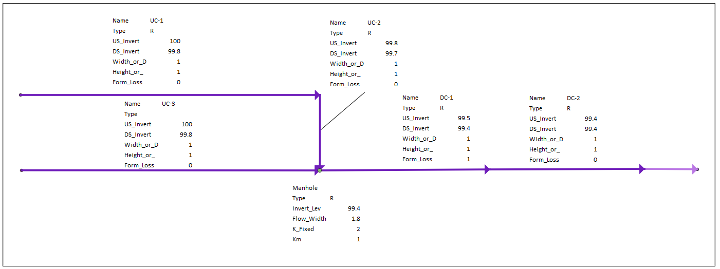
Figure 7: Example Model 3 Network Schematic
The conduits are the same shape and the same dimensions but have different invert levels as specified in the table below. All parameters for the manhole and other parts of the network are identical.

The resulting simulated loss values are presented in Figure 8.

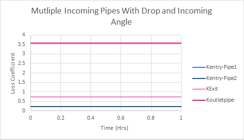
Figure 8: Example Model 3 Results-loss Coefficients

Example 3 - Entry Losses

This time the flow area in the manhole is 3.57m² and 1m² in the adjacent culvert whilst the flow is 1m³/s for Q_p and 2m³s^-1 for Q_om. Therefore, V_m equals:
And V_p:
From this:

This matches the losses for both incoming pipes as shown in figure 8.

Example 3 - Exit Losses

A'_m is 3.57m² respectively. Therefore, K^exit:

The calculated losses match the losses calculated by the TUFLOW presented in Figure 8.

Example 3 - Outgoing Conduit Losses

In this model we have two incoming pipes, one with an 90 degree angle between the incoming and outgoing conduit and one with zero. Recall that:

With Qf calculated as:
Q_p is set to 1m³s^-1 and Q_om to 2m³s^-1. Q_f is equal to 0.5m³s^-1. For the incoming conduit with an angle of 90 degrees, K_θ is therefore:

For the incoming conduit with an angle of 0 degrees, K_θ is therefore:

We also have a drop between the incoming and outgoing pipes. K_drop which represents losses due to this drop is calculated as follows:
and:

Therefore, K_outletpipe is:

The calculated value matches that presented in figure 8 for the downstream conduit loss.

Storage chambers

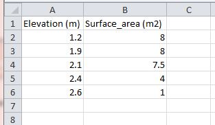
Storage, including storage chambers or floodplain storage, can be manually defined using a 1d_na (1d_tab_empty) node that has an assigned elevation versus surface area table. For the purpose of this page, manmade storage chambers have been discussed although the method is the same for all applications.

An example of a chamber:

www.humes.com.au

Methodology

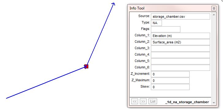
• Import 1d_na node.
• Assign the name of the elevation vs area csv.
• Specify the names for the elevation and surface area columns

storage_chamber.csv


For more information on storage nodes see Section 5.10.3 Storage Nodes (User Defined NA Tables) within the TUFLOW manual.


Any further questions please email TUFLOW support: support@tuflow.com

Back to 1D Hydraulic Structures