Difference between revisions of "1D Manholes"
Tuflowduncan (talk | contribs) |
|||
| (46 intermediate revisions by 3 users not shown) | |||
| Line 1: | Line 1: | ||
| − | |||
| − | |||
| − | |||
| − | |||
| − | |||
=Introduction= | =Introduction= | ||
| − | Manholes are typically chambers used to provide one or all of the following; maintenance access, change in culvert direction, connections and change in culvert dimensions. By default, manholes are automatically created within TUFLOW at all | + | Manholes are typically chambers used to provide one or all of the following; maintenance access, change in culvert direction, connections and change in culvert dimensions. By default, manholes are automatically created within TUFLOW at all conduit nodes, any manually created manhole will override the automatically created manhole. |
| − | Manholes are used at | + | Manholes are used at conduit junctions to dissipate energy due to: <br> |
| − | *Expansion/contraction of flow within the manhole chamber and outlet | + | *Expansion/contraction of flow within the manhole chamber and outlet conduits. |
| − | *Change in direction of the | + | *Change in direction of the conduits (i.e. a bend/deflection). |
| − | *Change in height, width or diameter and/or invert level of the adjoining | + | *Change in height, width or diameter and/or invert level of the adjoining conduits. |
<br> | <br> | ||
| − | The presence of a manhole at a junction point will override the exit loss of any | + | The presence of a manhole at a junction point will override the exit loss of any conduit discharging into the manhole and entrance loss of any conduit coming out of the manhole. <br> |
<br> | <br> | ||
| − | There are 3 types of manholes: | + | There are 3 types of manholes which can be specified in the 1d_mh_* layer: |
*"C" for circular chambers. | *"C" for circular chambers. | ||
*"R" for rectangular chambers. | *"R" for rectangular chambers. | ||
| − | *"J" for junctions without a chamber | + | *"J" for junctions without a chamber. |
<br> | <br> | ||
| − | =Losses= | + | =Manhole Losses= |
| − | When modelling conduit pipe flows, the head losses that the flow in pipe are subject to are made up of major losses (or friction losses) and minor losses (or local losses). Major losses are caused by forces between the flow and wetted perimeter of the conduit. Minor losses are caused by disruption to the flow due to bends, cross-sectional changes, fittings such as manholes and steps in the bed profile. Major losses are represented through the specification of a friction coefficient. The representation of minor losses, particularly | + | When modelling conduit pipe flows, the head losses that the flow in pipe are subject to are made up of major losses (or friction losses) and minor losses (or local losses). Major losses are caused by forces between the flow and wetted perimeter of the conduit. Minor losses are caused by disruption to the flow due to bends, cross-sectional changes, fittings such as manholes and steps in the bed profile. Major losses are represented through the specification of a friction coefficient. The representation of minor losses, particularly for gravity networks, is at manholes and requires separate treatment. The default TUFLOW/Estry manhole loss approach uses the Engelund method explained in section 5.12.5.4 of the [https://downloads.tuflow.com/_archive/TUFLOW/Releases/2018-03/TUFLOW%20Manual.2018-03.pdf TUFLOW user manual] although it is also possible to use a more simplified fixed manhole headloss approach too using the global <font color="blue"><tt>Manhole Default Loss Approach</tt></font> command or specifying within the '1d_mH_*' layer in the Loss_Approach attribute. The Engelund approach provides an automatic method for determining the loss coefficients as presented below. Of note is that the coefficients are recalculated every timestep, and therefore vary depending on the flow distribution between inlet and outlet conduits and the depth of water within the manhole. The losses represented are as follows: |
| − | + | <br> | |
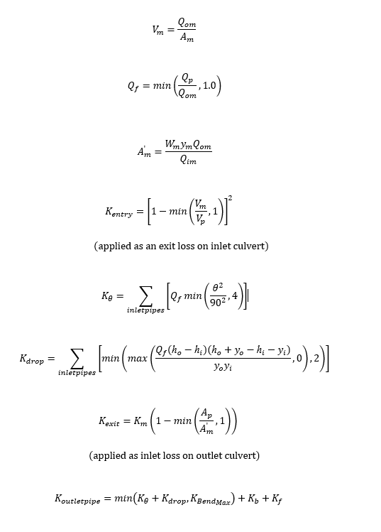
<li>'''K<sub>entry</sub>''' covers the expansion of flow within the manhole at the outlet of an inlet conduit. The coefficient is applied as the exit loss of the inlet conduit. | <li>'''K<sub>entry</sub>''' covers the expansion of flow within the manhole at the outlet of an inlet conduit. The coefficient is applied as the exit loss of the inlet conduit. | ||
| − | <li>'''K<sub>Ɵ</sub>''' represents the losses due to a change in direction (i.e. a bend) between inlet and outlet conduits. | + | <li>'''K<sub>Ɵ</sub>''' represents the losses due to a change in direction (i.e. a bend) between inlet and outlet conduits. K<sub>Ɵ</sub> is determined automatically by TUFLOW based on the angle of the digitised lines of the conduits. For the inlet conduit the last two vertices of the line are used and for the outlet conduit the first two vertices. |
<li>'''K<sub>drop</sub>''' is the loss coefficient due to a change in invert level and conduit height between inlet and outlet conduits. | <li>'''K<sub>drop</sub>''' is the loss coefficient due to a change in invert level and conduit height between inlet and outlet conduits. | ||
<li>'''K<sub>Ɵ</sub>''' and '''K<sub>drop</sub>''' are added and applied as an energy loss for each outlet conduit. | <li>'''K<sub>Ɵ</sub>''' and '''K<sub>drop</sub>''' are added and applied as an energy loss for each outlet conduit. | ||
| − | <li>'''K<sub>exit</sub>''' covers the contraction from the manhole and re-expansion of flow within the entrance of an outlet conduit. It is applied as an entrance loss of the outlet. | + | <li>'''K<sub>exit</sub>''' covers the contraction from the manhole and re-expansion of flow within the entrance of an outlet conduit. It is applied as an entrance loss of the outlet.<br> |
| − | <li>'''K<sub>m</sub>''' is the user-defined manhole exit coefficient. | + | <li>'''K<sub>m</sub>''' is the user-defined manhole exit coefficient. <br> |
| − | + | <br> | |
| − | The resulting headloss value is then applied, when sub-critical flow is experienced, to the standard head loss equation, i.e. dh = K*V<sup>2</sup>/2g. Where K is the loss coefficient, V is the conduit velocity and g the gravitational constant. The equations used for the Engelund loss approach are provided below: | + | The resulting headloss value is then applied, when sub-critical flow is experienced, to the standard head loss equation, i.e. dh = K*V<sup>2</sup>/2g. Where K is the loss coefficient, V is the conduit velocity and g the gravitational constant. The equations used for the Engelund loss approach are provided below:<br> |
<br> | <br> | ||
| − | [[File:Engelund Equations.PNG]] | + | [[File:Engelund Equations.PNG|500px]] |
<br> | <br> | ||
| Line 47: | Line 42: | ||
'''W<sub>m</sub>''' = Flow width in manhole (1d_mh width attribute) <br> | '''W<sub>m</sub>''' = Flow width in manhole (1d_mh width attribute) <br> | ||
'''y<sub>m</sub>''' = Depth of water in manhole <br> | '''y<sub>m</sub>''' = Depth of water in manhole <br> | ||
| − | '''A<sub>m</sub>''' = Flow | + | '''A<sub>m</sub>''' = Flow area in manhole <br> |
| − | '''A'<sub>m</sub>''' = Effective flow | + | '''A'<sub>m</sub>''' = Effective flow area in manhole <br> |
'''A<sub>p</sub>''' = Flow area of conduit <br> | '''A<sub>p</sub>''' = Flow area of conduit <br> | ||
'''K<sub>m</sub>''' = Manhole Loss Parameter (1d_mh Km attribute) <br> | '''K<sub>m</sub>''' = Manhole Loss Parameter (1d_mh Km attribute) <br> | ||
| Line 55: | Line 50: | ||
'''K<sub>Bendmax</sub>''' = Upper limit to sum of K<sub>θ</sub> and K<sub>drop</sub> (1d_mh K_Bend_Max attribute) <br> | '''K<sub>Bendmax</sub>''' = Upper limit to sum of K<sub>θ</sub> and K<sub>drop</sub> (1d_mh K_Bend_Max attribute) <br> | ||
<br> | <br> | ||
| − | + | There are three worked examples of the application of the Engelund method applied to a simple model for the following scenarios at the following pages: | |
| − | <li>Single Incoming/Outgoing Pipe with no angle and no drop | + | <li>[[Manhole_Simple_Loss_Example#Example 1: Single Incoming/Outgoing Pipe with No Incoming Angle or Drop|Single Incoming/Outgoing Pipe with no angle and no drop]] |
| − | <li>Single Incoming/Outgoing Pipe with incoming bend and drop in levels | + | <li>[[Manhole_Simple_Loss_Example#Example 2: Single Incoming/Outgoing Conduit with Incoming Bend and Drop in Invert Levels|Single Incoming/Outgoing Pipe with incoming bend and drop in levels]] |
| − | <li>Multiple Incoming Pipes with incoming bend and drop in levels | + | <li>[[Manhole_Simple_Loss_Example#Example 3: Multiple Incoming Conduits with Incoming Bend and Drop in Invert Levels|Multiple Incoming Pipes with incoming bend and drop in levels]]<br> |
| − | |||
| − | |||
| − | |||
| − | |||
| − | |||
| − | <br> | ||
| − | |||
| − | |||
| − | |||
| − | |||
| − | |||
| − | |||
| − | |||
| − | |||
| − | |||
| − | |||
| − | |||
| − | |||
| − | |||
| − | |||
| − | |||
| − | |||
| − | |||
| − | |||
| − | |||
| − | |||
| − | |||
| − | |||
| − | |||
| − | |||
| − | |||
| − | |||
| − | |||
| − | |||
| − | |||
| − | |||
| − | |||
| − | |||
| − | |||
| − | |||
| − | |||
| − | |||
| − | |||
<br> | <br> | ||
| − | + | In the case of the fixed headloss approach, the 1d_mh_* K_Fixed attribute is applied to the standard head loss equation, i.e. dh = K*V<sup>2</sup>/2g on the outlet conduit(s).<br> | |
<br> | <br> | ||
| − | = | + | =Manhole Storage= |
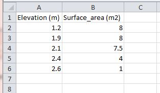
| − | + | Storage, including shaft storage, storage chambers or floodplain storage, can be manually defined using a 1d_na (1d_tab_empty) node that has an assigned elevation versus surface area table. For the purpose of this page, manmade storage chambers have been discussed although the method is the same for all applications. <br> | |
| − | |||
| − | |||
| − | |||
| − | |||
| − | |||
| − | |||
| − | |||
| − | |||
| − | |||
| − | |||
| − | |||
| − | |||
| − | |||
| − | |||
| − | |||
| − | |||
| − | |||
| − | |||
| − | |||
| − | |||
| − | |||
| − | |||
| − | |||
| − | |||
| − | |||
| − | |||
| − | |||
| − | |||
| − | |||
| − | |||
| − | |||
| − | |||
| − | |||
| − | |||
| − | |||
| − | |||
| − | |||
| − | |||
| − | |||
| − | |||
| − | |||
| − | |||
| − | |||
| − | |||
| − | |||
| − | |||
| − | |||
| − | |||
| − | |||
| − | |||
| − | |||
| − | |||
| − | |||
| − | |||
| − | |||
| − | |||
| − | |||
| − | |||
| − | |||
| − | |||
| − | |||
| − | |||
| − | |||
| − | |||
| − | |||
| − | |||
| − | |||
| − | |||
| − | |||
| − | |||
| − | |||
| − | |||
| − | |||
| − | |||
| − | |||
| − | |||
| − | |||
| − | |||
| − | |||
| − | |||
| − | |||
| − | |||
| − | |||
| − | |||
| − | |||
| − | |||
| − | |||
| − | |||
| − | |||
| − | |||
| − | |||
| − | |||
| − | |||
| − | |||
| − | |||
| − | |||
| − | |||
| − | |||
| − | |||
| − | |||
| − | |||
| − | |||
| − | |||
| − | |||
| − | |||
| − | |||
| − | |||
| − | |||
| − | |||
| − | |||
| − | |||
| − | |||
| − | |||
| − | |||
| − | |||
| − | |||
| − | |||
| − | |||
| − | |||
| − | |||
| − | |||
| − | |||
| − | |||
| − | |||
| − | |||
| − | |||
| − | |||
| − | |||
| − | |||
| − | |||
| − | |||
| − | |||
| − | |||
| − | |||
| − | |||
| − | |||
| − | |||
| − | |||
| − | |||
| − | |||
| − | |||
| − | Storage, including storage chambers or floodplain storage, can be manually defined using a 1d_na (1d_tab_empty) node that has an assigned elevation versus surface area table. For the purpose of this page, manmade storage chambers have been discussed although the method is the same for all applications. <br> | ||
<br> | <br> | ||
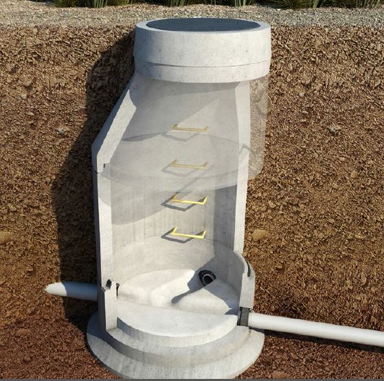
'''An example of a chamber:'''<br> | '''An example of a chamber:'''<br> | ||
| Line 256: | Line 66: | ||
<br> | <br> | ||
'''Methodology'''<br> | '''Methodology'''<br> | ||
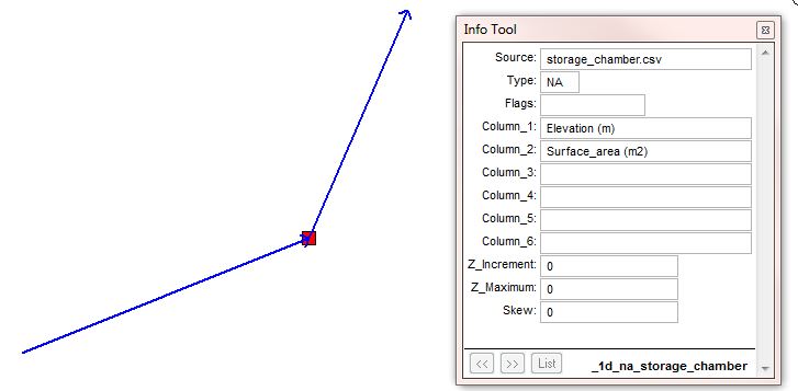
| − | *Import 1d_na node. | + | *Import the 1d_na node layer. |
| − | *Assign the name of the elevation vs area csv. | + | *Assign the name of the elevation vs area csv file. |
| − | *Specify the names for the elevation and surface area columns | + | *Specify the names for the elevation and surface area columns held within the csv file. |
<br> | <br> | ||
[[File:Storage_chamber_MI.JPG|border|600px]] | [[File:Storage_chamber_MI.JPG|border|600px]] | ||
| Line 266: | Line 76: | ||
[[File:Storage_chamber_csv.JPG|border|400px]] | [[File:Storage_chamber_csv.JPG|border|400px]] | ||
<br> | <br> | ||
| − | + | For more information on storage nodes see Section 5.11.4 ''Storage Nodes (User Defined NA Tables)'' within the [https://downloads.tuflow.com/TUFLOW/Releases/Latest/TUFLOW%20Manual.pdf| TUFLOW user manual]. If you have any further questions about manholes or any other aspect of TUFLOW functionality, please email TUFLOW support: [mailto:support@tuflow.com?Subject=TUFLOW%201D%20manholes%20help support@tuflow.com] | |
| − | For more information on storage nodes see Section 5. | ||
| − | |||
| − | |||
| − | |||
<br><br> | <br><br> | ||
| − | + | {{Tips Navigation | |
| + | |uplink=[[ TUFLOW 1D Channels and Hydraulic Structures | Back to 1D Channels and Hydraulic Structures]] | ||
| + | }} | ||
Latest revision as of 16:45, 1 March 2024
Introduction
Manholes are typically chambers used to provide one or all of the following; maintenance access, change in culvert direction, connections and change in culvert dimensions. By default, manholes are automatically created within TUFLOW at all conduit nodes, any manually created manhole will override the automatically created manhole.
Manholes are used at conduit junctions to dissipate energy due to:
- Expansion/contraction of flow within the manhole chamber and outlet conduits.
- Change in direction of the conduits (i.e. a bend/deflection).
- Change in height, width or diameter and/or invert level of the adjoining conduits.
The presence of a manhole at a junction point will override the exit loss of any conduit discharging into the manhole and entrance loss of any conduit coming out of the manhole.
There are 3 types of manholes which can be specified in the 1d_mh_* layer:
- "C" for circular chambers.
- "R" for rectangular chambers.
- "J" for junctions without a chamber.
Manhole Losses
When modelling conduit pipe flows, the head losses that the flow in pipe are subject to are made up of major losses (or friction losses) and minor losses (or local losses). Major losses are caused by forces between the flow and wetted perimeter of the conduit. Minor losses are caused by disruption to the flow due to bends, cross-sectional changes, fittings such as manholes and steps in the bed profile. Major losses are represented through the specification of a friction coefficient. The representation of minor losses, particularly for gravity networks, is at manholes and requires separate treatment. The default TUFLOW/Estry manhole loss approach uses the Engelund method explained in section 5.12.5.4 of the TUFLOW user manual although it is also possible to use a more simplified fixed manhole headloss approach too using the global Manhole Default Loss Approach command or specifying within the '1d_mH_*' layer in the Loss_Approach attribute. The Engelund approach provides an automatic method for determining the loss coefficients as presented below. Of note is that the coefficients are recalculated every timestep, and therefore vary depending on the flow distribution between inlet and outlet conduits and the depth of water within the manhole. The losses represented are as follows:
The resulting headloss value is then applied, when sub-critical flow is experienced, to the standard head loss equation, i.e. dh = K*V2/2g. Where K is the loss coefficient, V is the conduit velocity and g the gravitational constant. The equations used for the Engelund loss approach are provided below:

Where:
Qp = Flow in Conduit
Qim = Total flow into manhole
Qom = Total flow out of manhole
yi = Height of inlet conduit
yo = Height of outlet conduit
hi = Inlet conduit invert
ho = Outlet Conduit invert
θ = Angle in degrees of inlet conduit relative to outlet conduit(θ = 0° "when the culverts are in line," θ=90° when the outlet culvert is at right angles)
Qp = Flow in conduit outlet
Wm = Flow width in manhole (1d_mh width attribute)
ym = Depth of water in manhole
Am = Flow area in manhole
A'm = Effective flow area in manhole
Ap = Flow area of conduit
Km = Manhole Loss Parameter (1d_mh Km attribute)
Kb = Bend Loss Coefficient (1d_nwk Form_loss attribute)
Kf = Fixed Loss (1d_mh K_Fixed attribute)
KBendmax = Upper limit to sum of Kθ and Kdrop (1d_mh K_Bend_Max attribute)
There are three worked examples of the application of the Engelund method applied to a simple model for the following scenarios at the following pages:
In the case of the fixed headloss approach, the 1d_mh_* K_Fixed attribute is applied to the standard head loss equation, i.e. dh = K*V2/2g on the outlet conduit(s).
Manhole Storage
Storage, including shaft storage, storage chambers or floodplain storage, can be manually defined using a 1d_na (1d_tab_empty) node that has an assigned elevation versus surface area table. For the purpose of this page, manmade storage chambers have been discussed although the method is the same for all applications.
An example of a chamber:
Methodology
- Import the 1d_na node layer.
- Assign the name of the elevation vs area csv file.
- Specify the names for the elevation and surface area columns held within the csv file.

storage_chamber.csv

For more information on storage nodes see Section 5.11.4 Storage Nodes (User Defined NA Tables) within the TUFLOW user manual. If you have any further questions about manholes or any other aspect of TUFLOW functionality, please email TUFLOW support: support@tuflow.com
| Up |
|---|
