FMA Challenge 2
Introduction
The FMA Challenge models are example TUFLOW models submitted by BMT WBM for the Floodplain Management Association 2-Dimensional Model Challenges, 2012.
This Wiki page assumes an intermediate to advanced user level. If you haven't already completed FMA Challenge 1, please see the FMA Challenge 1 page.
This challenge model investigates a tidally influenced floodplain and riverine system along the Californian Coast. More information is available in the document "FMA Challenge 2 Documention.TUFLOW.docx" that is provided withing the ZIP file download.
All three challenge models are presented as a fully functional examples, allowing you to review the model setup, run the model and review results.
This model specifically shows:
- Tidal influences on floodplains and riverine systems;
- Variation in results due to 2D cell resolution and whether or not the model should contain a 1D component;
- The usage of a trd file to specify grid cell resolution and time steps;
- Looped batch files to run through scenarios; and
- The differences between two different 2D solvers, TUFLOW classic and TUFLOW GPU.
A key investigation of this FMA Challange is the performance of the differing 2D solution methods (CPU and GPU) in representing measured flood levels during a historical event.
Data for this model is provided in a variety of different GIS compatible formats. Download the dataset that matches the GIS software you are using:
Relevant Tutorials
It may be useful to revisit some of the following tutorials:
- General 2D modelling - Tutorial Module 1
- 2D topography modification - Tutorial Module 2
Model Setup
This section provides an overview and discussion of the model domain setup.
It is at your discretion which GIS package, text editor and method of model simulation to use (batch mode or within the text editor). All files required to setup and run the models are available within the download package. You have the choice of running with shape file or mif for usage in ArcGIS/QGIS or Mapinfo respectively.
This model does not require a licence dongle to run.
Grid Setup and Cell Size
A series of north-south oriented (10, 15 and 30m resolution) fixed grid domains have been developed over the coastal and estuarine study area.
When conceptualising the model domain, a fully 2D solution is preferable over a 1D/2D linked representation provided the 2D resolution of the primary flowpath/s is sufficiently fine. 'Sufficiently fine' is somewhat loosey defined as representing the channel with at minimum 4 fixed grid cells. Here, the 30m fixed grid resolution was determined sufficiently detailed to represent the river bathymetry.
For this model the upper sections near the two inflows are not represented well, especially the northern Tributary Inflow. However, this is unlikely to have an adverse effect on the objectives of the modelling, but would affect the comparison to the high water marks near these inflows.
As there is no 1D/2D linking, Challenge 2 provided an opportunity to provide some comparisons between our two different 2D solvers. Results from TUFLOW (finite difference implicit solution) and TUFLOW’s GPU Module (explicit finite volume GPU solver over a grid) are presented.
As with FMA Challange 1, variable model cell sizes have been simulated using the powerful event and scenario functionality of TUFLOW.
The grids investigated are as follows:
| 2D Domain | Active 2D Cells/Elements |
|---|---|
| 10m (grid) | 727,865 |
| 15m (grid) | 323,364 |
| 30m (grid) | 80,842 |
Note on Runtimes
There is a series of batch files provided with the demo model that give the choice of running only the 15m and 30m grid resolutions or all three. Due to the size of the model and large number of cells for the CPU only 10m case, it may take up to 24hrs of 'real time' to run on your computer. If you don't want to run the 10 m case then just run either 'run_all_001.bat' or '_run_all_CPU_001.bat'. Further details are provided in the Readme.txt within the runs directory.
Current benchmarching of runtimes for the CPU vs GPU respectively has found that the GPU simulations are typically 20-30 times faster than the CPU for this demo model. For models with a much larger number of cells >10 million the benefit of the GPU increases dramatically with CPU/GPU runtime speed increases over 100. Further detail on the hardware benchmarking conducted on FMA Demo Model 2 is provided here.
Simple Manning’s n / Topography Test
The initial runs were carried out using the same Manning’s n over the entire model over a coarse resolution grid (30m).
The topography for these runs did not include any special provision for incorporating the levee and road embankments. The elevation sampling of the DEM was simply based on inspecting the DEM at the models’ elevation points. At this stage no 3D breaklines along the embankment crests were used to ensure the crest of the elevation was correctly represented by the models’ elevations.
Simulations were carried out using a constant roughness initially, followed by variable roughness as defined by the NLCD Land Cover GIS layer and 3D breaklines of the levee and road embankments visible in the DEM and aerial photo. This scenario (we envisage) would probably be representative of the present day conditions, and not representative of the 1964 flood event conditions.
The NLCD GIS layer was read directly by TUFLOW and Manning’s n values assigned to the different land covers as tabulated below. The water/river n value of 0.02 is considered at the lower end of typical n values for rivers based on numerous 2D model calibrations. Typically for the lower reaches of coastal rivers the in-bank n value is 0.022 to 0.025 with an acceptable range considered to be (0.02 to 0.03). In upper reaches, away from tidal influences, n values tend to be higher (0.025 to 0.04) for perennial rivers. Possible reasons for the low n value could be due to the river bathymetry accreting since 1964 (we assume the bathymetry provided is based on more recent surveys), or the inflows maybe high.
The n values used are presented in the table below:
| Material ID | Manning's n | Description |
|---|---|---|
| 11 | 0.04 | Dummy Open Water - Overwritten by digitised polygon |
| 21 | 0.05 | Developed |
| 22 | 0.08 | Developed |
| 23 | 0.1 | Developed |
| 24 | 0.2 | Developed |
| 31 | 0.03 | Barren Land(Rock/Sand/Clay) |
| 41 | 0.05 | Deciduous Forest |
| 42 | 0.05 | Evergreen Forest |
| 43 | 0.06 | Unknown |
| 52 | 0.1 | Shrub/Scrub |
| 71 | 0.1 | Grassland/Herbaceous |
| 81 | 0.04 | Pasture/Hay |
| 82 | 0.05 | Cultivated Crops |
| 90 | 0.1 | Woody Wetlands |
| 95 | 0.1 | Emergent Herbaceous Wetlands |
| 101 | 0.02 | Water/Sand/Silt |
Model Calibration
The NLCD land cover provided a poor representation of the in-bank river section when compared with the DEM and aerial photography. The river section was therefore digitized to replace the NLCD representation in the river. A general comment overall was that the NLCD land cover was not always in agreement with the aerial photo and somewhat poor in its accuracy and resolution.
For the levee and road crests, GIS breaklines were digitized along the crests, and elevations sampled from the DEM (refer 2d_zsh_ridges_001). Ideally, ground surveys of these hydraulic controls would be available to ensure the crest is accurately modeled. TUFLOW reads the GIS breaklines and interpolates the crest elevation to the nearest 2D cell elevations to ensure the embankment height is correctly modeled.
In general the comparison with the high water marks tends to be higher overall, but the distribution of flow has improved with less water travelling to the southern tidal entrance. In a few areas it is worse such as in the images below. In the images the red values are the 1964 HWMs, and the black the calculated peak levels. In these areas the presence of the embankments has a strong influence on the calibration results. To test this influence a further scenario removing two critical embankments was carried out as discussed further below.


Removal of Major Embankments Scenario
To test the effect of completely removing the embankments in the images above, the 15m and 30m TUFLOW models were used. Initially the 30m model was run as this is a quick running model so good for an initial sensitivity tests.
The embankments were removed by digitizing the polygons shown in grey in the images below, and using TUFLOW’s Z Shape functionality that creates TINs within the polygons whose perimeters are merged with the surrounding ground levels to erase the embankments. Within the demo model, the embankment removal can be run using the scenario EMB. With this scenario applied, TUFLOW will modify the topography by calling the layer 2d_zsh_remove_ridges_001_R.shp as shown in the tgc file.
The images below for the initial 30m grid run show the levels at the high water marks with and without the embankments at the two locations previously discussed. The red values are the 1964 HWMs, the blue values the without embankments scenario and the black values in brackets for the with embankments case previously discussed. An improvement in the calibration results tends to result.
In conclusion, we would summarise that some of the key embankments within the study area either did not exist at the time of the 1964 event or were of a lower height or configuration.


Challenges
No unexpected “challenges” for Challenge 2, but it is worth noting the challenges that arise in calibration exercises. Sometimes there is an expectation that models should be able to reproduce recorded levels to within a very small tolerance. In these situations there needs to be a good understanding/appreciation by both the client and the modeller of the uncertainties and reasons for discrepancies; and the acceptable tolerances between the modeling and recorded observations accordingly set.
Are Manning’s n Values the Same for 1D and 2D models?
Generally Manning’s n values are very similar for 1D and 2D schemes. Where there is rapid changes in flow direction and magnitude (eg. at a structure, sharp bend or embankment opening), fully 2D schemes will simulate energy losses associated with the change in flow patterns, whereas 1D schemes either require user specified energy losses (eg. a structure) or artificially increasing Manning’s n. In these situations 1D schemes may utilize higher Manning’s n values than 2D schemes. Conversely, 2D schemes typically apply no side wall friction, so if there is significant wall friction a 2D scheme may require a slightly lower Manning’s n than a 1D scheme.
Calibration Challenges
Key challenges to note when calibrating are discussed below (this is not an exhaustive list but is a starting point!):
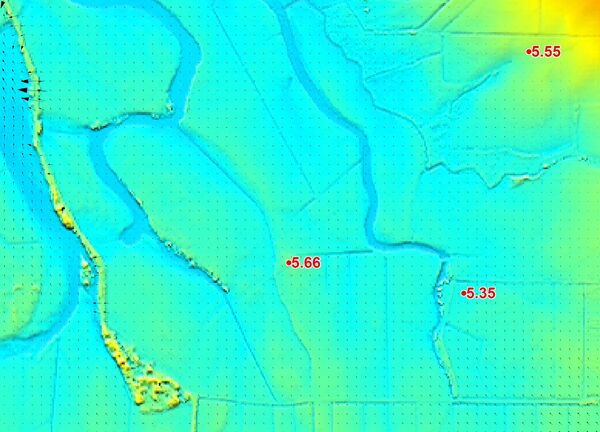
- Recorded levels can themselves be quite uncertain. They should preferably be rated as to their accuracy and the type of flood mark noted with the recording. For example, a water mark in the wall of a house is a reliable, accurate mark of the peak water level; while a debris level is simply an indication that the flood was at least this high (debris marks may not be at the peak of the flood). Scanning through the high water marks in this study would indicate some inconsistencies. For example, in the northern end of the study area the 5.35 HWM in the image below is upstream of the 5.66 HWM. Either the 5.35 is low and/or the 5.66 is high. If the accuracy of the HWMs can’t be established, then as a generalization, the modeler should err on the high side in case the flood mark was not recorded at the flood peak.
- The modeller should NOT adopt unrealistic parameter values (eg. excessively low or high Manning’s n values) for the sole purpose of achieving a good calibration. It is invariably the fact that there are other uncertainties causing the discrepancy when unrealistic Manning’s n values are used. Unrealistic Manning’s n values or other parameters (eg. high eddy viscosity) distort the results and are a sure sign that there is something else wrong.
- Levees, roads, railways and other embankments can have a major influence on the flood behavior. Those embankments that overtop should be ground surveyed along their crests and the crest height correctly represented in the model’s elevations. Often for calibration events the height or presence of the embankments is not known accurately and this needs to be taken into account in the ability of a model to reproduce flood marks.
- The inflows to a model for historical floods often have a high degree of uncertainty, and are the most common reason for a poor calibration. The precise distribution spatially and temporally of the rainfall is not known (sometimes there is little or no rainfall data), and/or the rating curve at a model boundary has significant uncertainties. The significant uncertainties associated with developing model inflows should be understood and appreciated by modeler and client. Ideally, one or more recorded hydrographs would be available to the modeler to verify that the model can reproduce the shape and timing of the flood. If a hydrologic model is being used to generate the inflows, then the calibration exercise should be a joint exercise in calibrating both the hydrologic and hydraulic models.
- Inaccurate topography has become less of an issue in recent years with the advent of more accurate aerial surveys. However, the bathymetry of the main flowpaths, and storage capacity of floodplain backwaters, needs to be accurately represented if the model is to have any chance of reproducing flood marks. If these areas have permanent water and/or dense vegetation, the aerial surveys are still incapable of accurately surveying them, so other forms of survey maybe required. If accurate surveys are not available for these areas, this adds to the uncertainty in the modeling and the ability of the model to reproduce historical flood events. There is also the issue of using contour data instead of the raw terrain data to create the DEM as highlighted in our Challenge 1 discussion.
- Structures are often poorly represented due to lack of data. For example, in the aerial photograph below for Challenge 2 there appears to be some structures (which has two calibration points in the vicinity). However, with no details provided, the structure below can only be modeled as a simple opening in the embankment with no allowance for bridge decks, etc.


Caveats
In summary, the TUFLOW 15m No Embankments simulation provided the best calibration.
Conclusion
In this challenge, we explored a tidally influenced floodplain and riverine system. From this, we gained a better understanding of how cell resolution affects results and when it is suitable to neglect 1D components, how to use a looped batch file to run through scenarios, and an understanding of comparison between the CPU and GPU TUFLOW solvers.
Congratulations on finishing Challenge 2! Please click here to return to the main page.