TUFLOW 1D Channels and Hydraulic Structures

Introduction

The objective of the following pages is to supplement the TUFLOW manual and provide additional modelling guidance on 1D hydraulic channels.

1D Channel Types

1d_nwk channels represent open channels, hydraulic structures, operational structures and other flow controls. A channel is either digitised as a line or point with the relevant hydraulic properties entered into the appropriate GIS attributes, details for this can be found within the links below or the TUFLOW manual.

Open Channels

Channel Type	Description of page contents
Open Channels	This page contains information on basic commands, error checking and common check files used.

Structures

The table below contains a complete list of 1D structures available within TUFLOW, including logic control structures.

Channel Type	Description of page contents
Culverts	1D-2D connections, flow regimes, operational control and common check files used.
Bridges	Loss theory, irregular shaped bridges and common check files used.
Weirs	*under construction*
Gates	*under construction*
Pumps	Pump attributes, 2D-2D & 1D-2D configurations, Estry setup, depth-discharge database and 1D results file.
Pits	Pit inlet types, depth-discharge data sources, modelling advice.
Manholes	Losses and storage chambers.

Special Channels

Channel Type	Description of page contents
M Channels	*under construction*
Q Channels	*under construction*
Operating Controls (*.toc)	*under construction*

Common Questions Answered (FAQ)

What is the difference between 1d_pit and 1d_nwk layer for pits?

The 1d_pit layer is a newer and simplified version of the 1d_nwk layer for pits.

1d_pit

• Assumes default values for any of missing attributes that are described for the 1d_nwk pits layers.
• Does not have invert attributes. The upstream invert is assumed to be the ZC elevation of the connected 2D SX cell, as such the "L" flag is not supported. The downstream invert needs to retrieve its value from the connected 1d_nwk channel.
• The nodal area assumes the default, the downstream pit channel node has its nodal area automatically assigned based on the connected 1d_nwk channel segments that have the UCS attribute set to “true”. The applied nodal area can be confirmed in the .eof file.
  
• Virtual pipes can only be setup with the 1d_pit layer.

1d_nwk

• Used for models that needs to deviate from the default approaches.

How can I read approach-capture flow curves for on-grade pits into TUFLOW?

TUFLOW currently doesn't support the use of approach-capture flow curves directly. To get around this, pit depth-flow curve relationship can be derived as follows:

• Select a few representative slope increments for the project area and do a Manning's equation calculation for each to calculate the gutter flowrates for incrementally increasing flow depths.
• Multiply the above flows by the % value in the on grade curve. This turns the % capture vs. flow curve into a depth vs. flow relationship.
• Repeat for different gutter shapes.

Should I model culverts in the 1D or 2D domain?

This largely depends on the size of the culvert in comparison with the cell size. Most commonly culverts are modelled within the 1D domain, however, with more computational power given by GPU devices, cell sizes are getting smaller and it might be beneficial to model bigger culverts in 2D. If the culvert is an important aspect of the study, it is always recommended to model it in number of ways by either using different methods and/or different software and the afflux is cross-checked against a desktop analysis and hand calculations. None will be 100% right, but the intent here is to establish a verification of the preferred approach.

2D only approach

• Benefits:
  • Good stability and improved hydraulic behaviour at the culvert entrance/exit.
  • The expansion loss (exit loss) can be explicitly handled in 2D provided the 2D cell resolution is sufficiently fine to model the expansion of flow downstream of the culvert.
• Challenges:
  • The contraction loss (entry loss), which is related to the expansion of water after the vena-contracta and forms inside at the culvert inlet, won't be picked up well and some additional energy loss (form loss) might be needed to cover this.
  • Side and soffit wall friction are not modelled unless Manning's n varies with depth, i.e. increase Manning's n with depth to account for the missing Manning's n on the side and top surfaces.
  • The vertical walls not only create extra friction but also straightens the flow in the direction of the wall. Thin breaklines can be used to represent these walls in 2D, but it is likely to cause saw-tooth effect if sub-grid sampling (SGS) is not used, i.e. extra numerical head loss, if there are too few cells between the walls. SGS is recommended in this case.
  • Flow overtopping can be represented to some extent by assuming 100% blockage of layer 2 in a 2d_lfcsh, but the flow upstream and downstream before the culvert is overtopped is hard to model.

2D-1D-2D approach

• Benefits:
  • A more appropriate approach where the 2D cell size is greater than around half the total culvert width.
  • Contraction losses (entry losses) are handled better.
  • Flow overtopping can be modelled in 2D.
• Challenges:
  • Expansion losses (exit losses) are very dependent on the 2D cell resolution. A 2D cell size much larger than the culvert width will not reproduce the expansion losses very well (even with SGS) and the culvert's exit loss needs to cover this. A finer 2D cell size (several or more cells across the culvert) will reproduce the expansion losses much better and the culvert's exit loss need to be reduced to compensate it. This usually only happens for large 1D culverts with high velocities as there can be losses duplicated in the 2D on the exit side as the 2D flow expands (i.e. duplication of the exit/expansion loss). The latest release has a new feature to automatically adjust 1D culvert losses based on the 2D approach/departure velocities as what happens with a 1D-1D-1D arrangement. See this paper for more information.
  • HX connections may cause instability, especially with a skewed culvert outlet, but can produce better velocity patterns downstream of the culvert to model the expansion losses, which will be occurring in the 2D domain.
  • Given that the SX connection applies the flow going out of the 1D culvert as a source term without momentum, it is difficult to completely prevent the water from piling up. If required, wingwalls can be modelled as thin breaklines to help guide the water away. Using the SX boundary Z flag lowers other SX cells below the 1D culvert invert level and it can mitigate the water from piling up.

What entry/exit loss and contraction coefficients should I use for 1D culverts?

We don’t provide hard recommendations on the exit and entry losses to use for culverts as we have found different organisations around the world, typically government, have their own guidelines for different types of inlets configurations and require these to be used, for example, the Queensland Urban Drainage Manual (QUDM). However, it is very important to understand how losses are applied and that different 1D solvers may treat them differently. For cross-checking your results from any hydraulic modelling software, a simple calculation applying the entry and exit losses (allowing for any automatic adjustments as discussed below) to the computed head (V2/2g), plus allowing any surface roughness losses (Manning's equation) for longer culverts, is the best practice for culverts flowing in a sub-critical flow condition (i.e. downstream controlled flow).

For the entrance loss values, the approach should be to use values as quoted in the literature or guidelines for the inlet shape and design unless there is evidence to use another value (e.g. comparison with reliable calibration data would indicate different energy losses).

For the exit loss a value of 1.0 is recommended in nearly all situations provided losses are being adjusted every timestep. A value of 1.0 with adjusted losses is derived from the fluid flow physics (momentum or energy conservation) for expanding flow and will be the most precise approach for modelling exit losses or to apply a bend loss to the approach/departure channel if these are modelled in 1D.

Occasionally there are situations where non-standard entrance and exit loss values are needed. A good example is if the approach or departure flow is skewed to the culvert direction. In these situations there may also be a significant bend (energy) loss occurring as the water changes direction entering or leaving the structure. To account for this the modeller may need to increase the entrance and/or exit loss values.

By default, TUFLOW adjusts the entrance and exit losses of 1D structures flowing sub-critical every timestep based on the approach/departure velocities for 1D-1D-1D and with a new feature in the 2020-10-AA build for 2D-1D-2D. The entrance losses are adjusted based on an empirical relationship from flume testing whilst the exit loss equation is theoretically derived as mentioned above - see Section 5.7.6 from the 2018 TUFLOW Manual. The modeller should be familiar with the approach taken by the software they are using as some software either don't adjust for approach/departure velocities at structures (will overestimate losses using standard values) and some may apply a limiting loss thereby not allowing the losses to sufficiently reduce.

TUFLOW, by default, allows the losses to reduce to effectively a zero loss coefficient (i.e. 0.0001). A zero loss occurs where the approach and departure velocity is the same as the structure velocity. For example, a clear-spanning bridge over a concrete lined channel with the water level below the bridge deck will experience no energy losses until the bridge deck is surcharged so if your software is applying unadjusted or limited energy loss coefficients there will be an unrealistic energy loss at the structure for flow below the bridge deck. For culverts, in most cases there will be some losses as it is rare that the channel is of identical shape and slope to the culvert with usually the culvert being more constrictive and therefore a higher velocity so the adjusted coefficients are nearly always non-zero. At the other extreme is flow from or into a near still body of water (e.g. a lake or the ocean). In this situation the loss coefficient(s) will not be reduced and the maximum energy loss possible should occur.

If the default adjust losses approach is used (Structure Losses == ADJUST) the recommendations are to use industry guidelines for the entrance loss coefficient based on the shape/design of the inlet (these coefficients are typically based on a near zero approach velocity), and to use 1.0 for the exit loss coefficient. This applies to 1D culverts connected to 1D channels. The adjusted entrance and exit losses can be viewed over time in the _TSL layer, see Table 13-2 from the 2018 TUFLOW Manual.

Since the 2020-10-AA release, TUFLOW has a new (beta functionality) to have the losses automatically adjusted for linked 1D culverts and other structures connected to 2D domains through SX links (Structure Losses SX == ADJUST), see Section 6.2 from the 2020-10 Release Notes. Note, it is likely this setting will become the default in a future TUFLOW release once beta testing and further benchmarking is completed.

The other values to consider for modelling culverts are the inlet contraction coefficients used when the flow is upstream controlled flow should this occur. Typically the TUFLOW default values for these values should be used unless the inlet shape and design indicates otherwise.

Should I model pits as R or Q type?

Q pits are recommended for modelling kerb inlets, catchpits, drains, etc., provided that appropriate y-Q curves are available. TUFLOW automatically extends the y-Q curve for higher depths based on the orifice equation. Under downstream controlled flow regime it reverts to a drowned condition.
When using the R pit, whilst the pit is free-falling into the pipe system below (most of the time until the system surcharges), entrance/exit losses don't apply, because the flow is inlet controlled. The R pit would be using the weir equation for unsubmerged flow or orifice flow for submerged flow and could be a poor representation of the pit flow behaviour, especially if the pit also has a grate and other non-rectangular characteristics.

How to model pipe network with some pipe data missing?

In situations where the complete pipe network is not modelled there are numerous common approaches adopted by modellers:

• Use direct rainfall boundary conditions, model all inlets, only model the larger pipes in the pipe network. Where a small pipe is being omitted, connect the flows from the inlet to the main pipe network using virtual pipes functionality. Only the location of the inlet pits are needed, they can be approximated and sometimes lumped representation of the pits. This approach is especially good if the pipe network does not surcharge back to the overland flow anywhere or only in a minor way.
• Use lumped hydrology inflows. Only model the main pipe network and connected inlets (excluding the smaller features). Apply the flows directly to the pits either with:
  • 1d_bc QT polygon boundaries with a P flag. This automatically distributes the total flow to all the pits within the polygon.
  • 2d_sa boundaries with a "Read GIS SA PITS" command. The flow is applied to the ground surface rather than directly into the manhole. Some of the flow will surcharge out of the pits if the downstream pipe capacity is exceeded.

How can I get more inflow into the pipe system?

A shallow depth can occur in the pit inlet cell and underestimate the depth at the entrance to the pit, restricting the amount of flow entering the pit. This can happen specifically for larger cell sizes. Different options to capture more water from 2D cells into the pits are available based on the TUFLOW engine. Both approaches aim to account for changes in ground elevation that occur at a finer scale than the 2D cell resolution:

• TUFLOW HPC - use Sub-Grid Sampling (SGS) - this approach samples underlying DEM with finer resolution and represents the true topography more accurately guiding water into the pits.
• TUFLOW Classic - use "Pit Default Road Crossfall" command to increase the depth at Q pits based on the crossfall slope of the road cross section. TUFLOW calculates the water depth that is used by the Pit Inlet Database using an adjacent side triangle depth approach, instead of the actual cell flow depth.

How is flow through the culvert calculated?

Computationally, information is passed between the 1D and 2D on the half timestep:

• Flow through the culvert is calculated based on the water levels at the inlet/outlet and the assigned flow regime. The volume is extracted/added to the 2D boundary cells on the half timestep.
• On the next full timestep the 1D and 2D shallow water equations are applied to move water through their respective domains.

What should I do if 1D pump doesn't convey as much flow as expected and/or seems to be unstable?

A couple of things can be checked:

• The inlet of the pipe has to be fully submerged, otherwise the pump will shut down and there will be no flow through the pump.
• Add extra storage to the node upstream of the pump with 1d_na table or 1d_nwk type NODE through ANA attribute.
• Try reasonably smaller 1D timestep.
• If using non-operational pump (P), check if the depth discharge relationship is appropriate. If outlet of the pipe is lower than inlet, the pump will always try to pump at full capacity.
• Consider using operational pump (PO), where the pump would switch off if the water level upstream gets below the pump soffit.

How BB bridges automatically switch between pressure flow and being drowned out?

TUFLOW considers the top of the XZ or HW table as the soffit level. If the downstream water level exceeds the soffit level, TUFLOW does the pressure flow calculation using default K = 1.56. It compares the velocity calculated by the pressure flow equation and by the form loss calculation based on LC table and uses the smaller one. The _TSF and _TSL layers can be used to find out the regime/form loss values used for BB bridges:

• "P": pressure flow
• "D": ds water level > the soffit level, but it applies normal flow because the normal flow equation predicts smaller velocity
• " ": ds water level < the soffit level, normal flow

Should I model bridges in the 1D or 2D Domain?

The recommended approach typically depends on the study objectives and if the channel upstream and downstream of the bridge is modelled in 1D or 2D. To preserve the momentum as accurately as possible the bridge should be modelled in the same dimension as the channel, e.g. 1d_nwk bridge if the channels is in 1D and 2d_bg or 2d_lfcsh if the channel is modelled in 2D.
In 2D, the expansion/contraction losses are modelled based on the topography and don't need to be estimated as attributes as for 1D modelling. Also, for higher flows where the bridge is overtopped, 2D is preferable approach.

What is the difference between downstream and upstream controlled flow?

Downstream control means a change in downstream water level will cause a change in upstream water level. Upstream control means the upstream water level is insensitive to the downstream water level and usually indicates the occurrence of supercritical flow.

How do negative "M", "N" and "R" values deactivate 1D cross-sections?

When negative “M” values are used to deactivate 1D cross-sections, it changes the flow area, wetted perimeter, hydraulic radius, and the conveyance, while keeping the storage width unchanged. It is like inserting a thin plate at the middle of the channel, as shown in the figure below. This approach is preferred to retain the storage in the system but reduce the conveyance (e.g., off-stream storage not contributing to conveyance or sections either side of a constriction to generate better approach/departure velocities if using the Total Area approach).


When using negative “N” (Manning’s n) or “R” (relative resistance factor) to deactivate the 1D cross-sections, it reduces both the flow area and the storage width, as shown in the figure below.

Calculating a 1d_bc Head-Discharge Curve

There is no automatic way of creating a Head-Discharge curve for 1d_bc HQ boundaries. However, the condition to be satisfied for a normal depth is the Manning’s equation. So the HQ depth should be set up with elevation and the discharge calculated from Manning’s equation (including Area and Hydraulic Radius for each elevation point) and can be calculated manually in a few steps:

1. Set the model up your ESTRY model using a dummy downstream level boundary (e.g. a HQ boundary with no name, an error will be reported however the required check file will have been produced, otherwise any boundary will work) and run the model in test model (-t) so that check files are produced.
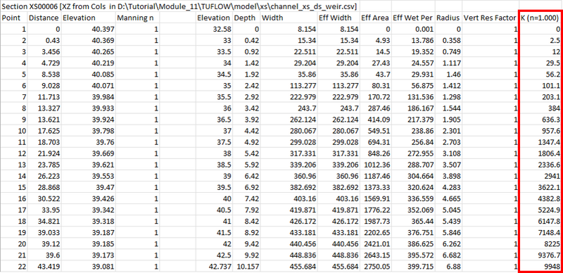
2. From the check folder, open the *_1d_ta_tables.csv file.
3. Find the entry for the most downstream cross-section (directly upstream of the 1d_bc HQ point). The *_1d_ta_tables.csv will contain a table of hydraulic parameters. The K entry highlighted is the cross-section conveyance in m³/s and is calculated as:
   K = 1/n * A * R^2/3
   Where
   • A is the Eff Area
   • R is the Radius
   
   
   
   
4. Determine a representative slope (S), this could be taken from the last two cross-sections.
5. Calculate the downstream Discharge (this is the same as calculated discharge from Mannings equation):
   Q = K * SQRT(S)
   Where:
   • S is a representative slope value for the downstream reach.
   • K is obtained from the 1d_ta_tables.csv
6. Use the Elevation (Head) vs Discharge pairs to populate the HQ table.

Why is the maximum 1D water level higher than 2D water level?

TUFLOW calculates storage at 1D nodes (including manholes) and calculates flux at pipe mid-sections. The storages at the manholes are saved in the format of ‘elevation vs nodal area’ tables, which you can check from the .eof file:

The change in water volume in a manhole is calculated based on the inflow from the pit above (if there is one) and the inflow/outflow from the connected pipes. The change in water level is then calculated based on the change in volume and the nodal area at that elevation.

TUFLOW extends the ‘elevation vs nodal area’ table by 5 m (as you can see from the last 2 numbers in the table above), which allows for the calculation of pressurised pipe flow when a manhole is drawn. If the maximum 1D water level is higher than the dem, that means the manhole was drawn and pressurised during the peak of the flood.

Up
Back to TUFLOW Modelling Guidance