Introduction

TUFLOW’s Advection Dispersion (AD) Module is an extension of the TUFLOW Classic/HPC engines. It adds to the hydrodynamic capabilities of TUFLOW Classic/HPC by simulating depth-averaged, two and one-dimensional constituent fate and transport. An example of such a constituent might include salinity. Both dissolved and particulate constituents can be simulated. TUFLOW AD takes depth and velocity fields computed by the TUFLOW Classic and HPC solvers and uses this information, together with initial and boundary conditions, to simulate the advection and dispersion of user-defined constituents.

TUFLOW AD is specifically oriented towards such analyses in systems including coastal waters, estuaries, rivers, floodplains and urban areas. The AD module is discussed in detail in the TUFLOW Advection Dispersion Manual.

Model Development

Setting Up a New Model

The steps below describe the process for setting up a TUFLOW AD model. It is assumed that the user is familiar with TUFLOW Classic/HPC and that the folder structure for TUFLOW has been setup with all required files. The user should run the TUFLOW Classic/HPC model without the AD module first to make sure that it is appropriately configured and stable.

Create a TUFLOW AD control file with the extension .adcf
Use a text editor to create an empty .adcf file and save it to the “runs” folder.
Set up the AD global database (.csv file).
Set up the TUFLOW AD global database in the “bc_dbase” folder which defines the constituent of interest and a number of characteristics, for example the decay rate and dispersion coefficient. The resulting file should look similar to the below:
In the .adcf file use the "AD Global Database" command to set the location of the global database as follows.
AD Global Database == ..\bc dbase\my_ad_global_dbase.csv
Set up the boundary condition tables (.csv file(s)) to define the time-varying constituent concentrations at any input boundaries.
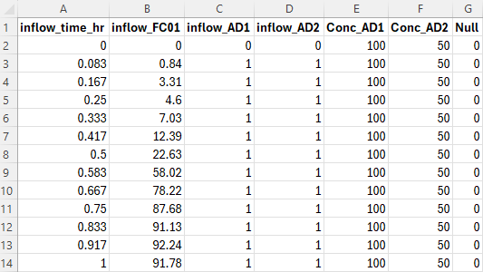
- Set up the constituent boundary condition table(s) in the “bc_dbase” folder . For example in the below, the time-varying concentration of constituents Conc_AD1 and Conc_AD2 are set:
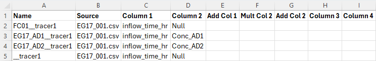
Set up up the boundary condition database (.csv file)
- Set up the boundary condition database in the “bc_dbase” folder that references the tables set up in the previous step.
- In the .adcf file use the "AD BC Database" command to set the location of the bc database as follows.
  AD BC Database == ..\bc dbase\my_ad_bc_dbase.csv
Setup up TUFLOW to activate the AD module (.tcf file)
- In the .tcf file use the command "AD Control File" to set the location of the adcf and activate execution of the AD module as follows.
  AD Control File == ad_run.adcf
Run the model
Run TUFLOW as normal. The AD module will be called and appropriate constituent result output files written.

Example Models

Example TUFLOW AD models, including settling and decay, are available via the TUFLOW Example Model Dataset.

Common Questions Answered (FAQ)

How can the Advection Dispersion module be used to determine the time of concentration in a 1D-2D TUFLOW model?

The Advection Dispersion module can track particles and determine the time of concentration by simulating how a particle of water travels from an upstream to a downstream location. However, the AD module is only available for 2D domains and cannot directly operate within a 1D channel.

To utilise the AD module in this case, the 1D channel would need to be converted into a 2D domain using a Quadtree grid. This conversion involves refining the 2D cells within the channel to smaller sizes, ensuring the model accurately represents the flow behaviour. Once this modification is complete, the AD module can provide detailed insights into particle travel times and help demonstrate the effects of reprofiling or attenuation measures on downstream areas.

Can TUFLOW generate 2D Plot (Time-Series) Output for Advection Dispersion results?

Currently, TUFLOW does not support 2D Plot (Time-Series) Output for Advection Dispersion results at specific point locations.

However, results can be extracted using output zones. Defining smaller output zones allows high-frequency data to be generated for areas of interest while managing file sizes efficiently. Multiple output zones can also be used to monitor widely separated locations.

How can initial tracer concentrations and SGS parameters be managed in the Advection Dispersion module?

Initial tracer concentrations can be applied to dry cells, and these concentrations are mobilised as the cells become wet during a simulation. The initial water level in dry cells is set as the bed elevation plus the Cell Wet/Dry Depth. This depth determines the initial tracer volume available for advection once the cell becomes inundated.

When SGS (Sub-Grid Sampling) is used, the initial water volume is derived from a pre-calculated “level vs cell volume” curve. Tracer concentrations are distributed across this calculated volume. This ensures accurate representation of tracer movement, even in partially wet cells.

How can the Advection Dispersion module be used to determine water residency time?

The Advection Dispersion module in TUFLOW can be used to calculate water residency time by modelling it as a scalar variable. This approach provides a method for tracking the duration water has spent within a specific area, such as a wetland, and is visualised in the model output as a time-based scalar field. This approach has some limitations:

Output Capabilities: While TUFLOW supports various output formats (e.g., XMDF, DAT, NC), extracting detailed time-series data for specific constituents at individual locations may require additional post-processing. The current AD module does not explicitly support direct Point Output (PO) functionality for constituent data.
Post-Processing Requirements: To obtain detailed residency time information at specific points, output zones may be required along with refined post-processing techniques. Defining output zones allows high-frequency scalar data to be captured in areas of interest, which can then be analysed to estimate residency times.
Engine-Specific Features: Unlike the TUFLOW FV engine, which includes a particle tracking module for explicit tracking of water age, the fixed grid engine’s AD module relies on scalar-based methods to approximate residency time. For calculating water residency time with the AD module, properly configuring scalar outputs and planning post-processing steps are essential for accurate results.

How can the Advection Dispersion module simplify firewater containment modelling?

The Advection Dispersion module in TUFLOW can simplify firewater containment modelling by using passive tracers to track firewater flow and concentration. Instead of running separate simulations for rainfall and firewater scenarios, the AD module enables a single simulation where tracers represent the firewater. This approach reduces modelling complexity while maintaining accuracy.

For example, a model with direct rainfall over the entire domain applies a passive tracer via 2d source area (2d_sa) polygons. The output can be set up to identify areas with tracer concentrations above a certain threshold, distinguishing firewater extents from other inundated areas. Areas outside of this represent zones with zero tracer concentration. Tracers can also include decay and settling parameters for added flexibility. This method not only simplifies the process but also ensures compliance with CIRIA (Construction Industry Research and Information Association) guidance by integrating rainfall and firewater scenarios into a single simulation.

What guidance is available for Non-Newtonian Mixing Exponents and Dispersion Coefficients in the TUFLOW Advection Dispersion Module?

The Non-Newtonian Mixing Exponents (m, o, and p) were introduced in the 2023-03-AC release to improve how TUFLOW models non-Newtonian fluids. These exponents control how yield stress and density change as fluid concentration varies.

Previously, using a single exponent for all properties was ineffective for fluids with high solids content. For example, yield stress can increase rapidly with small changes in solids, while density changes more gradually.

It is recommended that these exponents range between 1 and 5. However, the optimal values depend on the specific fluid being modelled, and should be selected based on the fluid’s properties. TUFLOW does not provide specific default values.

For dispersion coefficients:

In pure water, the longitudinal dispersion coefficient (KL) is usually between 6 and 13, and the transverse dispersion coefficient (KT) is between 0.15 and 1.6.

Extremely high values, like 7500, only occur in special conditions such as estuarine environments with a halocline and are not typical for most cases.

Currently, there is no guidance for dispersion coefficients when mixing pure water with non-Newtonian fluids. Suitable values should be determined based on laboratory tests or studies specific to the fluid being modelled.

What are the limitations of the Advection Dispersion module when modelling Non-Newtonian flow through 1D elements in TUFLOW?

When using the Advection Dispersion module for non-Newtonian flow in models that include 1D elements, the following simplifications and limitations apply:

Flow Calculation:

The flow through 1D elements (e.g., culverts) is calculated based on the assumption of pure water.
Non-Newtonian properties, such as viscosity or yield stress, are not considered in the 1D engine. This simplification can lead to an overestimation of flow rates when dealing with non-Newtonian fluids.

Tracer Transport:

By default, the concentration of the non-Newtonian fluid is passed instantly from the upstream to the downstream node in 1D channels.
The transport equation is not calculated for the 1D elements. This can cause an underestimation of travel time for non-Newtonian fluids, particularly in long 1D elements.

These limitations mean that while the AD module can be used in models with 1D elements, it does not fully capture the complexities of non-Newtonian fluid behaviour in those elements. If higher accuracy is required, 2D elements where non-Newtonian properties are more comprehensively represented may be considered.

Up
Back to TUFLOW Modelling Guidance

Advection Dispersion Modelling

Contents