Python Library TUFLOW Results
Introduction
For the 2016 version of TUFLOW a new output format for time-series was made available, this has the following changes from previous versions:
- Combines the 1D results, 2D plot outputs and new reporting location data
- The outputs are stored in a separate Plot folder in the TUFLOW results directory
- .tpc (TUFLOW Plot Control file links to data in csv and gis folders
- Has additional Node and Channel information files contain connectivity information
This is the default approach for the 2016 version but can be modified with the TUFLOW command "Output Approach == Pre 2016" (refer to the manual for more information on this command.
To make this data easier to work with an open source python library has been created and made available. This allows the user to load results and then interact with these. This library does not have any plotting functionality directly, with the returns typically being arrays (e.g. time and flows) however, the examples below give some examples using common plotting libraries such as matplotlib.
Getting the TUFLOW results python library
You can find the TUFLOW_results.py (previously TUFLOW_Results2016.py) on the QGIS plugin repository, on the TUFLOW support GitHub repository or if you have QGIS and the TUFLOW plugin installed, you will already have it on your computer.
- QGIS plugin repo: https://plugins.qgis.org/plugins/tuflow/
- If you select Download Latest and save the .zip file, the TUFLOW_results.py sits inside the .zip file.
- GitHub: QGIS plugin https://github.com/TUFLOW-Support/QGIS-TUFLOW-Plugin
- If you select Clone or Download and then select Download Zip and save the .zip file, the TUFLOW_results.py sits inside the .zip file.
- QGIS
- If you have QGIS2 with the TUFLOW plugin installed via the plugin repository, the TUFLOW_results.py sits within: C:\Users\<User Name>\.qgis2\python\plugins\tuflow
- If you have QGIS3 with the TUFLOW plugin installed via the plugin repository, the TUFLOW_results.py sits within: C:\Users\<User Name>\AppData\Roaming\QGIS\QGIS3\profiles\default\python\plugins\tuflow
- If you have QGIS2 with the TUFLOW plugin installed via the plugin repository, the TUFLOW_results.py sits within: C:\Users\<User Name>\.qgis2\python\plugins\tuflow
The TUFLOW python library does not need to be installed in python (through pip or otherwise) like other common modules, the TUFLOW_results.py file just needs to be in the same location as your python project.
Note it shouldn’t matter if you’re using python 2 or python 3.
Dependencies
The TUFLOW results library calls a number of python modules, these are:
- csv
- numpy
- os
- sys
Of these the csv, os and sys functionality should be available directly with the python install. Depending on the method used to install python, numpy may need to be installed. If installation of numpy is required, please refer to the numpy documentation http://www.numpy.org/.
Compatible Python Versions
The functionality has been developed for Python 2.7, but should be compatible with Python 3.5. Other versions of python are currently untested.
Usage
Import
This library is imported with the typical python syntax.
import TUFLOW_results
Initialise Results (ResData)
The results data functionality has a class defined, this is named ResData. An instance of the results can be initialised with the following syntax:
res = TUFLOW_results.ResData()
Defined Methods (Functions)
The following are the defined functions in the results data class (ResData).
Load Results
Results are loaded in with the syntax below.
error, message = res.Load(r'D:\TUFLOW\QGIS\test\plot\Plot_Example.tpc')
The two return arguments are:
- error (logical) set to True if an error has been encountered.
- message (string), if an error has occurred the message string will be populated with an error message.
Get Time-series
Time-series at a 1D, 2D or reporting location can be returned using the following syntax:
found, results, message = res.getTSData(<ID>,<domain>,<results type>,<geometry>)
The inputs to this are:
The return arguments are:
For example:
found, results, message = res.getTS('ds3','1D','Q','L')
Will return flow (Q) data for the 1D channel with ID ds3. The optional 'L' geometry indicates that this is stored on a line object in the GIS plot objects. Note As the time data typically does not change (this is not a return argument) but can be accessed by the res.times. See the examples below.
Long Profile Functions
When dealing with 1D long profile data, if a single 1D channel is specified the data for all channels downstream will returned. If two channels are specified, long profile data will only be returned for the channels between the specified channels.
Get Long Profile Connectivity (LP_getConnectivity)
This determines and stores the connectivity of the specified channels. This is used in later routines to determine the channels and nodes to plot for the long profile. The syntax is:
error, message = res.LP_getConnectivity(<US Channel ID>,<US Channel ID or None>)
The inputs to this are:
The return arguments are:
error, message = res.LP_getConnectivity('FC01.40',None)
Determines all the channels downstream of FC01.40.
error, message = res.LP_getConnectivity('FC01.40','ds3')
Determines the channels between FC01.40 and ds3, an error will be returned if these channels are not connected.
Get Long Profile Static Data (LP_getStaticData)
Once the connectivity between two channels has been determined, this routine can be used to get data that does not change between time-steps. This includes:
- distance information
- maximum data
- bed levels
The syntax is:
error, message = res.LP_getStaticData()
There are no input arguments as the channel connectivity is stored in the res.LP class. The return arguments are:
Get Long Profile Data (LP_getData)
This function gets data at a specific time. If looping through timesteps (e.g. for an animation) the channel connectivity and static data will not change between timesteps and therefore only the LP_getData will need to be repeated. The syntax is:
error, message = res.LP_getData(<data type>,<time>,<time search tolerance>)
The inputs to this are:
The return arguments are:
error, message = res.LP_getData('Head',1,0.01)
Returns the water level (head) data at time 1 hours using a search tolerance of 0.01 hours.
Other Attributes
Once initialised the ResData class also has a number of attributes associated with it as well as the defined functions described above, these are outlined in the table below.
| Attribute Name | Type | Description |
|---|---|---|
| script_version | string | Contains a version number of the TUFLOW results library, e.g. '2016-01-AA' |
| filename | string | The full filepath to the .tpc file. |
| fpath | string | The path of the folder which contains the .tpc file. |
| nTypes | integer | The number of data types that are stored in the dataset. |
| Types | list | A lists of the data types that are stored in the dataset. |
| LP | class (LP) | Contains Long profile information, connectivity, distances etc. |
| Data_1D | class(Data_1D) | The 1D results are all stored in this class. |
| Data_2D | class(Data_2D) | The 2D results are all stored in this class. |
| Data_RL | class(Data_RL) | The reporting location results are all stored in this class. |
| GIS | class(GIS) | This contains the information read in from the GIS Plot Layer csv files. |
| formatVersion | integer | The format version of the results as defined in the .tpc file. |
| units | string | The units as defined in the .tpc. E.g. "Metric" or "English" |
| displayname | string | The simulation name e.g. "M04_5m_001_2015" |
| Index | class(PlotObjects) | This contains data read from the "GIS Plot Objects" |
| nodes | class(NodeInfo) | Contains information on the 1D nodes, as read from the "1D Node Info" .csv file. |
| Channels | class(ChanInfo) | Contains information on the 1D nodes, as read from the "1D Channel Info" .csv file. |
| times | numpy ndarray | The active times. This is typically static, however calls to function getTS may cause this array to be updated (if the 1D or 2D outputs have a different output interval) |
Examples
These examples work with the Tutorial Model module 4 results. The tutorial model can be downloaded on the TUFLOW website.
Plot Flow in Channel
import os						#operating system functions
import sys						#system functions
import matplotlib.pyplot as plt
import TUFLOW_results

input_res = r'C:\TUFLOW\Models\Tutorials\QGIS\Complete_Model\TUFLOW\results\M04\2d\plot\M04_5m_001.tpc'

# initialise the results class
res = TUFLOW_results.ResData()

# Load the data and terminate if error returned
error, message = res.Load(input_res)
if error:
    print(message)
    sys.exit()
print('loaded')

#create a figure
fig = plt.figure() #create new figure
ax1 = fig.add_axes((0.10, 0.15, 0.85,0.75)) #add axis to figure

#Get flow data
chan_id = 'ds3' # this is the channel ID to use
found, results, message = res.getTSData(chan_id,'1D','Q','L')
if found:
	print('found requested data')
	# plot data
	ax1.plot(res.times,results,color='b',label='Flow - '+chan_id)
else:
	print(message)
	sys.exit()

# manage plot
ax1.set_xlabel('Time (hours)')
ax1.set_ylabel('Flow (m3/s)')
ax1.set_title('Example time-series - single location')
ax1.grid()
ax1.legend()
plt.show()
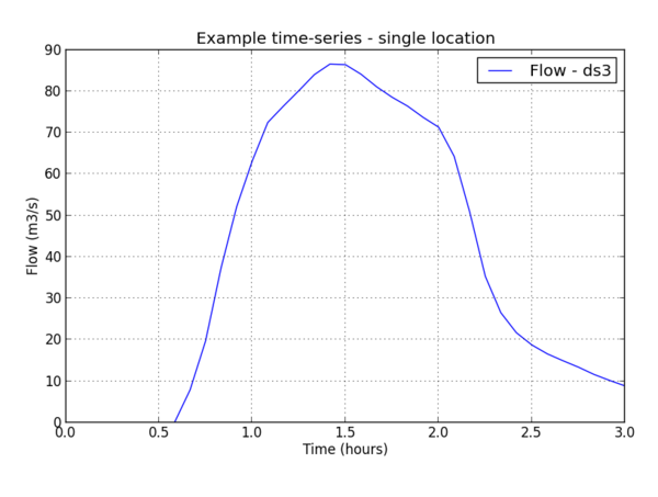
This will create a figure that looks like the above.
Plot Multiple Water Levels
In this example, it is assumed that the results data has been loaded as per the above.
#create plot
fig = plt.figure() #create new figure
ax1 = fig.add_axes((0.10, 0.15, 0.85,0.75)) #add axis to figure

# list of nodes to plot
node_ids = ['FC01.14.1','FC01.15.1','FC01.16.1','FC01.17.1']

#Get water level data
for node_id in node_ids: #for each node in the list above
	found, results, message = res.getTSData(node_id,'1D','H','P')
	if found:
		print('found requested data')
		# plot data
		ax1.plot(res.times,results,label='Level - '+node_id)
	else:
		print(message)
		sys.exit()

# manage plot
ax1.set_xlabel('Time (hours)')
ax1.set_ylabel('Water Level (mAHD)')
ax1.set_title('Example time-series - multiple locations')
ax1.set_ybound((38.,44.)) #overwrite the y axis bounds
ax1.grid()
ax1.legend(loc='lower right')
plt.show()
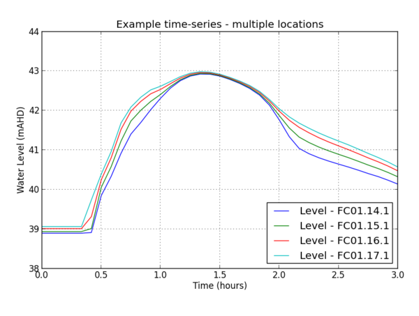 This will create a figure that looks like the above.
Dual Axis (flow and velocity) Plot
In this example it is assumed the results have been loaded as per example 1.
# specify channel to plot
chan_id = 'ds3'

#create plot
fig = plt.figure() #create new figure
ax1 = fig.add_axes((0.10, 0.15, 0.80,0.75)) #add axis to figure
ax2 = ax1.twinx() #create new axis with same x properties

#Get flow data
found, results, message = res.getTSData(chan_id,'1D','Q','L')
if found:
	print('found requested data')
	ax1.plot(res.times,results,color='b',label='Flow - '+chan_id)
else:
	print(message)
	sys.exit()

#Get velocity data
found, results, message = res.getTSData(chan_id,'1D','V','L')
if found:
	print('found requested data')
	ax2.plot(res.times,results,color='r',label='Velocity - '+chan_id)
else:
	print(message)
	sys.exit()

# manage plot
ax1.set_xlabel('Time (hours)')
ax1.set_ylabel('Flow (m3/s)')
ax2.set_ylabel('Velocity (m/s)')
ax1.set_title('Example time-series - twin axis')
ax1.grid()
h1, l1 = ax1.get_legend_handles_labels()
h2, l2 = ax2.get_legend_handles_labels()
ax1.legend(h1+h2, l1+l2, loc='upper left')
plt.show()
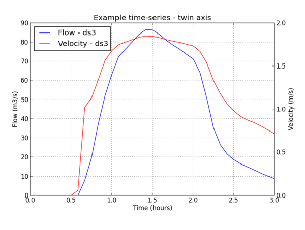
This will create a figure that looks like the above.
Long Profile Peak Levels
This also assumes that the data has been loaded as per example 1 above. The long profile data for all channels downstream of FC01.40 will be plotted.
us_chan = 'FC01.40' #upstream channel
ds_chan = None

#get connectivity between channels
error, message = res.LP_getConnectivity(us_chan,ds_chan)
if error:
	print(message)
	sys.exit()
else:
	print('LP connectivity determined.')

print('Get LP static data')
error, message = res.LP_getStaticData()
if error:
	print(message)
	sys.exit()
else:
	print('LP static data retrieved')

#create plot
fig = plt.figure() #create new figure
ax1 = fig.add_axes((0.10, 0.15, 0.85,0.80)) #add axis to figure

#plot data
# Max WL
ax1.plot(res.LP.dist_nodes, res.LP.Hmax,color='r',label = 'Max Water Level')

# Bed Level
ax1.plot(res.LP.dist_chan_inverts, res.LP.chan_inv,color='brown',linewidth = '3',label = 'Bed Level Level')

# manage plot
ax1.set_xlabel('Distance (m)')
ax1.set_ylabel('Level (mAHD)')
ax1.set_title('Example Long Profile - Peak Levels')
ax1.grid()
ax1.legend(loc='upper right')
plt.show()
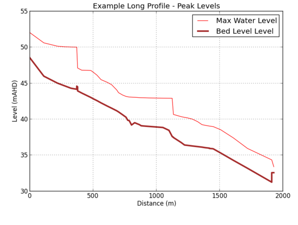
This will create a figure that looks like the above.
Other Versions
An older version of the library that is compatible with results from the 2013 version of TUFLOW (this is limited to the 1D results) is also available. This is currently undocumented, however, if you would like this please contact support@tuflow.com.
| Up |
|---|
