Tute M06 MI 2D lfsch Archive

In the following steps we will be adjusting the elevations of the road crest as well as using a 2D zsh layer to lower the zpt elevations at the location of the 2D bridge.

Method

Lower the 2D Elevations Through the Bridge Opening

1. Copy the 2d_zsh_M06_NorthRd_001 from Module_Data\Module_06\2D_Bridge folder into the TUFLOW\model\mi folder. We will use this layer to remove the road embankment at the 2D Bridge location.
2. Open the newly saved layer 2d_zsh_M06_NorthRd_001 in MapInfo and make it editable.
Observe the shape contained in this GIS layer. The polygon intersects the zpts where we want to modify the elevations and remove the road embankment. We will remove the embankment at this location by creating a GIS layer that tells TUFLOW to interpolate zpt elevations within the shape using the zpt elevations either side of the embankment. Additionally, the GIS layer will be designed such that TUFLOW does not use the zpt elevations where the two shapes intersect with the embankment. Refer to Section 4.4.9 and Table 4.8 of the 2010 TUFLOW manual for more information on this procedure.
3. Digitise four points snapped to each of the polygon nodes that are circled in the image below.
Tip: It is helpful to make nodes along the polygon perimeter visible by customising the layer properties in layer control. Before digitising points, ensure snap mode is turned on by hitting the S key.

4. We need to update the Z attribute of the points. Browse the table of the 2d_zsh_M06_NorthRd_001 layer using the New Browser tool. In the table browser, select the four points such that they are highlighted.
5. Use the Table >> Update Column tool to update the Z attribute of the points. Ensure the Table to Update: is Selection (the default) and the Column to Update is Z. Enter -99999 in the Value: box. Click 'OK' and you should see that the eight points in the browser table now show -99,999 as their Z attribute. These points tell TUFLOW to ignore the zpt elevations where the polygons intersect the embankment.

6. Save and export the table in .mid/.mif format. The 2D zsh at the bridge is now ready for TUFLOW.

Create the 2D Layered Flow Constriction

The following steps are used to create the 2D layered flow constriction - 2d_lfsch - that will represent the bridge in the 2D domain. The flow constriction layers provided here are mostly completed. If these were not provided, the method would be to import the "2d_lfsch_empty.mif" and "2d_lfsch_empty_pts.mif" files from the TUFLOW\model\mi\empty folder and save them in the TUFLOW\model\mi\ folder, renaming the files and beginning the edits in these new layers.

1. Copy the two 2d_lfsch layers from the Module_Data\Module_06\MapInfo\2D_Bridge folder into the TUFLOW\model\mi folder.
2. Start MapInfo and open the M04_5m_001.wor workspace located in the Complete_Model\TUFLOW\runs folder that is provided. This workspace is created by TUFLOW when a simulation is started, this contains all the MapInfo layers read into a TUFLOW simulation.
3. In MapInfo open the 2d_lfcsh_M06_bridge_001 layer from Step 7 and the Digital Elevation Model layer, DEM_M01, provided in theModule_Data\DEMs\Vertical_Mapper folder. The 2D cells within the layered flow constriction shape are those that we are going to modify to represent the layers of the bridge in the 2D model domain. We will first define the form loss and blockage associated with three layers in the polygon object. After we have defined the layer characteristics on the 2d_lfsch polygon object, we will then define the elevations at which each layer occurs using points.
4. Make the 2d_lfcsh layer editable and add the following attributes to the polygon shape, leaving other attributes unchanged.
   

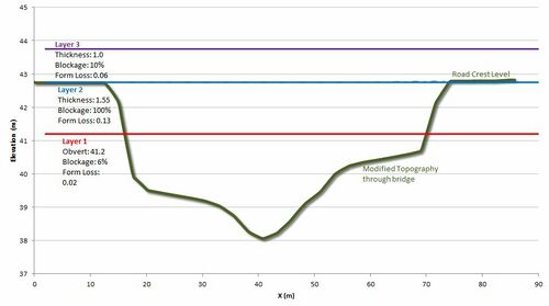
   Attribute	Value
   Invert	99999
   L1_pBlockage	6
   L1_FLC	0.02
   L2_pBlockage	100
   L2_FLC	0.13
   L3_pBlockage	10
   L3_FLC	0.06
   Notes	Northern_Bridge

The attributes are described fully in Table 4.21 of the 2010 TUFLOW manual. Note that L1, L2, and L3 refer to varying layers, as described in Section 4.7.2.3. We are setting:
• Enter an "Invert" value of 99999 to leave the Zpt levels unchanged (ie. use the Zpt elevations modified by the 2d_zsh layer above).
• Percentage blockage below the obvert of layer 1 to account for any blockages perpendicular to the direction of flow (in this case 6% to account for the average blockage due to the bridge piers).
• A Form Loss Coefficient (FLC) below the obvert of layer 1 (in this case to account for sub-grid scale losses around piers). Note that the treatment of the FLC is different depending on the object used to define the flow constriction, i.e. a line or a polygon. The reason for this is to permit the flow constriction to be independent of the model cell size. See Table 4.19 in the 2010 Manual for more information. In this case, a polygon has been used and the FLC specified is the form loss per metre length in the predominant direction of flow. FLC values are dependent not on the flow width, but on the length of travel in the direction of flow. Our intention for this study, is to apply a total FLC of 0.3 below the obvert of the bridge. The value entered is therefore 0.3 / 15m which gives a value of 0.02. Refer to latter sections of this tutorial for guidance on how to check the applied FLC.
• Blockage from the obvert level to the top of layer 2 (in this case 100% to account for the bridge deck).
• A form loss for layer 2, the bridge deck (in this case a total of 1.95 to account for the deck and the water level rising to and exceeding the deck). The attribute value entered is 1.95 / 15m giving a value of 0.13.
• A blockage from the top of the deck to the lop of layer 3 (in this case 10% to account for fence rails above the deck).
• A form loss from the top of the deck to the top of layer 3 (in this case 0.06 to account for sub-gird scale losses around the railings).
5. Open the 2d_lfcsh_M06_bridge_001_P layer and make it editable. This layer contains point data snapped to nodes on the layered flow constriction and will allow us to define the elevations at which the layers occur. We are using points along the perimeter of the shape because their use allows us to vary the height and depth of layers 1 to 3 within a single shape if required. For simplicity, in this tutorial we have left the bridge soffit and deck at a constant height however the point functionality can be modified if you wish to experiment. Most of the points are already provided together with their attributes. Finish the lfcsh points layer by digitising two points snapped to the nodes at the locations shown below and adding the following attributes:

   Attribute	Point 1	Point 2
   Invert	39.0	39.0
   L1_Obvert	41.2	41.2
   L2_Depth	1.55	1.55
   L3_Depth	1	1

Note that the invert level has been specified as 39 m. This is the height at which the piers start impact flow and also the height as which the flc and blockage will be implemented.

6. The above edits and layers result in the below bridge configuration:
   
7. Save and export the table in .mid/.mif format. The 2D bridge is now ready for TUFLOW.

Conclusion

The layered flow constriction layers have been created to model the new bridge on the northern road. Please return to the main page of module 6.