View Results in SMS 11.1 Archive
Introduction
In this page we will look at viewing TUFLOW results using SMS 11.1. This allows us to step through each output time and watch the flood as it progresses through the catchment. We will look at both scalar and vector data.
For information on SMS please visit the Aquaveo software website SMS Introduction. If you do not have a licence for SMS a 30 day trial can be obtained. To obtain a trial download the SMS 11.1 (full installation) from here Aquaveo Downloads. After installation, upon starting SMS for the first time select "request evaluation".
Opening Aerials
SMS can handle aerial photos in a variety of image formats (such as .ecw, and JPG). Images can be registered within SMS (see SMS tutorials / help for instructions). However, for this tutorial the registered images have been provided. If the SMS window you are working on does not already have the aerial photo loaded, follow the following step to load it:
You may be prompted to "Build Image Pyramids", this creates new images of the .jpg at a variety of resolutions for quicker redrawing. Select "Yes" if prompted.
Opening Results
To view results in SMS we need at least two files open. The first is the TUFLOW mesh, this contains information on the location, cells and elevations within the model. This data is contained in a 2D Mesh (.2dm file). Once this has been loaded the TUFLOW results can be loaded, the TUFLOW results can either be in either the .dat (1 results file format per output type) or .xmdf (one output file that contains all of the results).
TUFLOW also writes out a .sup file contains instructions for SMS to open the mesh first and the the TUFLOW results.
- To open all of the TUFLOW results from the menu toolbars select File | Open and navigate to the results directory (for the tutorial model, module 1 this is TUFLOW\Results\M01\2D\ Folder) and open the relevant .sup file. For module 1 this is M01_5m_002.all.sup file.
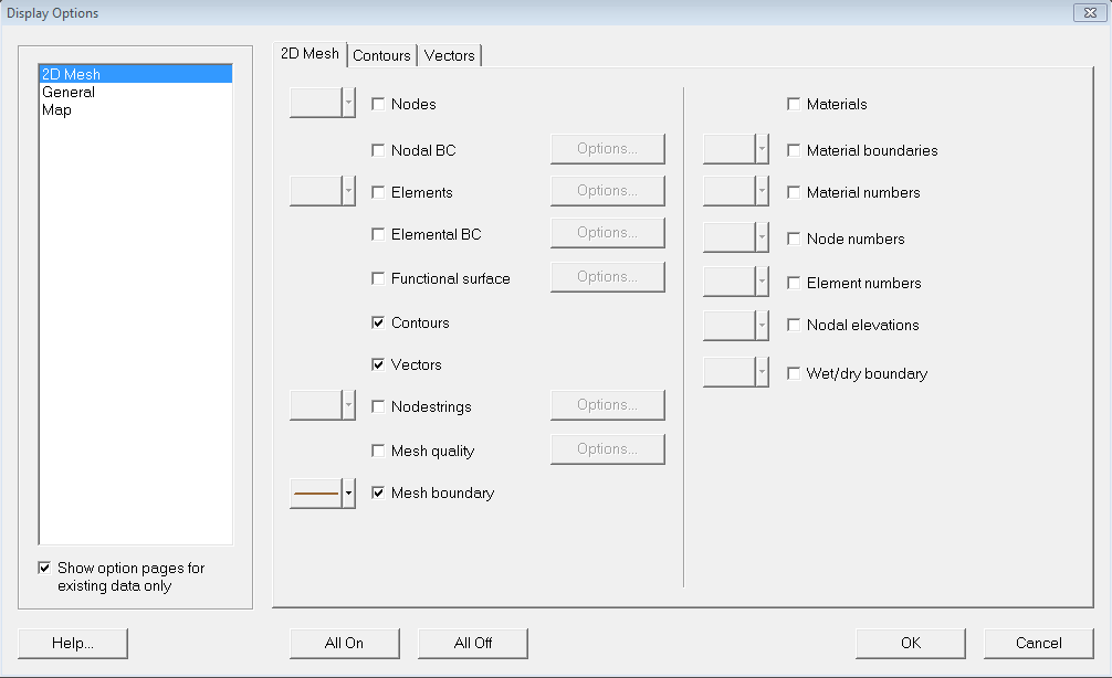
- To open the Display Options Dialog, in the menu items select Display | Display Options....
TIP: The shortcut key to bring up the Display Options dialog is Control + D. In the Display Options dialog, ensure that you are in the 2D Mesh module in the pane to the left. In the 2D mesh tab, you get a list of options ticking the check box will make an item visible. Turn everything off, except for the mesh boundary and the contours.
Once opened, the SMS view may (depending on defaults) look something like this. In the upper left is a project explorer, the TUFLOW results should now be listed here in Mesh Data. There should also be a list of available output times (every 5 minutes).

We have a large number of options for viewing results. To change what is displayed in the Map Area open the Display Options Dialog.

Viewing Scalar Data

To view the scalar dataset, ensure that the "contour" option is checked as per the image above. In the project window under Mesh Data is a list of the scalar and vector datasets available.
Scalar datasets are indicated by the icon "123" and vector datasets have 2 arrows as the icon. The image on the right shows a list of datasets that we turned on before running the TUFLOW tutorial simulation(Module 1).
If you look at the project explorer, under Mesh Data, there is a solution set for Module 01 (M01_5m_002). This solution set has three folders for the following categories of data:
- Maximum with a list of maximum value of the data in the entire duration
- Temporal with time varying values for the data
- Time with the times for peak V and peak h for each data
- Select the Depth dataset in Temporal folder.
- In the "Time Steps" window, select a timestep and use the up and down arrows to step through the results.
- Bring up the Display Options dialog, and select the "Contour" tab under 2D Mesh.
- Under Contour Method select 'Color Fill.
TIP: Normal Linear can be used to display contour lines only, and Color and Linear displays both contour shading and contour lines. - Select a colour ramp to suit
Contouring Options
There are numerous options for controlling how the scalar results display (colour profile, contour increment, transparency). This is controlled in the Contour tab in the Display Options dialog. A brief guide is given below, feel free to experiment.

Under "Color Ramp" you can choose the colour profile. There are numerous options here, feel free to experiment. In the image shown here, an Intensity Ramp varying from light blue to dark blue has been chosen.

In the Data Range section of the Display Options dialog there is a summary of the minimum and maximum data values for the selected dataset. For the TUFLOW Tutorial Model: Module 1, the results vary between 0.0 to 5.9 metres deep (approximately). A range can specified here, by checking the "Specify a range" option. In the image shown here an upper range of 4.0 metres has been set so that anything above this depth will display in the upper contour range (dark blue).
TIP: by specifying a range and un-checking "Fill Above" or "Fill Below" you can restrict the display range. For example, setting a minimum of 0.1m and un-checking "Fill Below" any depths less than 0.1m will not be displayed. A transparency can also be set in this dialog, this can make the aerial photo visible beneath the contouring.
Viewing Vectors
- To turn on the vectors, navigate to the 2D Mesh tab of the Display Options (Display | Display Options). Check the Vector item, as per the image below.
- Select the Velocity Vector vector item under Temporal folder in the project window, scroll through the time steps to view the vectors at each output time.
Vector Display Options
There are numerous option for controlling the size, shape and density of the vectors displayed. This page gives only a brief introduction, users are encouraged to experiment!
To open the vector options, navigate to the Display Options, select the 2D Mesh in the left hand pane, and then select the Vectors tab, as shown in the image below.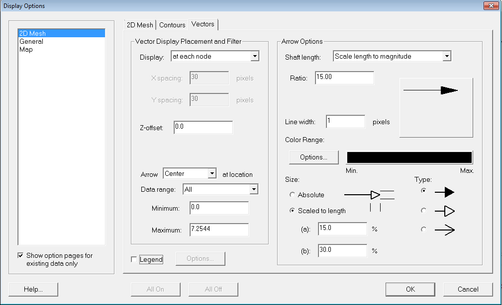
In this dialog you can control:- If the vectors are shown at each cell corner (Display: at each node) or on a regular grid (Display: on a grid).
- Vertical offset (Z offset)
- Tip a value of greater than 0 ensures the vectors appear on top of the contours.
- The data range (use this to restrict values)
- Arrow size, this can be fixed length or scale length to magnitude
- Tip scale length to magnitude is recommended for most result viewing
- Line width
- Colour
- Arrow head
- Set the following (as per the image above):
- Display: to 'at each node
- Shaft length: scale length to magnitude
- Ration: 15
Select Ok
The map display should look like the image below.


Advanced
For more information on viewing results in SMS, please see the SMS Tips.
For those progressing through the Tutorial Module 1, you can return to the tutorial module here.