Flood Modeller Tutorial Module02
Introduction
In this module, a proposed development is represented within an existing model by adding TUFLOW 1D pipe network elements, which are then linked with Flood Modeller Pro.
This will include:
- Modification of the floodplain topography through the creation of a 3D TIN surface.
- Revision of the land use.
- Addition of pipes and pits in ESTRY to represent the underground network.
- Linking of the pipe network in ESTRY with the Flood Modeller network.
- Introduction of an inflow into the pipe system.
- Addition of a river reach represented in ESTRY downstream of the Flood Modeller network.
GIS and Model Inputs
The steps required to modify each of the GIS inputs are demonstrated in QGIS using SHP and GPKG formats. Instructions for completing the module in ArcGIS or MapInfo are available on the archive page for Tutorial Module 02.
Define Elevations (Building a TIN)
The GIS layers necessary to modify the ground elevations to represent the proposed development are provided. This part of the tutorial demonstrates how a TIN is created from these GIS layers. The GIS defining the road crest level is also updated. Instructions are available below for the preferred GIS format:
Define Surface Roughness
The GIS layers necessary to modify the land use areas affected by the proposed development are provided. This part of the tutorial demonstrates how to populate the layer attributes to assign Manning’s n roughness values to each land use. Instructions are available below for the preferred GIS format:
Define Pipe Network
This part of the module creates the GIS layers that define the sub-surface pipe network. The inlets and pits of the pipe network are linked to the 2D domain. The pit inlet database is also created, linking the GIS layers to depth-discharge curves. Instructions are available below for the preferred GIS format:
Define Boundary Conditions
This part of the module demonstrates how an inflow can be applied directly to the pits of the pipe network. A GIS layer of the inflow boundary is provided. The existing Boundary Conditions Database is also modified to include these new inflows. Instructions are available below for the preferred GIS format:
Flood Modeller 1D/ESTRY 1D Link
This part of the module demonstrates how TUFLOW 1D (ESTRY) domains can be dynamically linked with Flood Modeller using "X1DH" and "X1DQ" links. Instructions are available below for the preferred GIS format:
The Flood Modeller 1D/ESTRY 1D link can be employed for a number of reasons, including:
- Inclusion of the pipe network and manhole modelling capabilities of ESTRY within a Flood Modeller – TUFLOW linked model (see Section 10.5 of the TUFLOW Manual for more details).
- Extension of a Flood Modeller network within ESTRY to overcome Flood Modeller node licence limits.
- Representation of a steeper tributary in ESTRY which can then be connected to the main river represented in Flood Modeller.
Flood Modeller and TUFLOW (ESTRY) nodes are considered linked if an ESTRY node in a 1d_nwk layer and a Flood Modeller node in a Read GIS X1D Nodes or Read GIS X1D Network layer are snapped together, or are within the snap tolerance distance specified.
ESTRY nodes are automatically generated at the upstream and downstream extremities of an ESTRY link, so manual generation of a node is not mandatory. If no node is manually added, the Flood Modeller–ESTRY link is assumed to be an “X1DH” link. If an ESTRY node is manually generated, the ESTRY node can have a 1d_nwk layer Conn_1D_2D attribute of either “X1DH” or “X1DQ”.
An "X1DH" link means a Flood Modeller 1D water level is applied at the ESTRY node (i.e. Flood Modeller sends ESTRY a water level and ESTRY sends back a +/- flow to Flood Modeller). An ESTRY "X1DH" link (the default) is typically used where ESTRY discharges into a Flood Modeller network. The "X1DH" link is applied to the Flood Modeller 1D network as a lateral inflow. The Flood Modeller 1D node connected to the ESTRY node by an "X1DH" connection must not be the end node of a reach.
An "X1DQ" link means a Flood Modeller inflow/outflow is applied at the ESTRY node (i.e. Flood Modeller sends ESTRY a +/- flow and ESTRY sends back a water level). This is more appropriate where a Flood Modeller network terminates and flows into an ESTRY model. The Flood Modeller 1D node at the end of an "X1DQ" connection must be an HTBDY unit, although it is not necessary for the HTBDY unit to contain any boundary data as this data is overridden by the water levels provided by TUFLOW.
Modify Simulation Control Files
With the input GIS layers modified, the next step is to update the TUFLOW control files and Flood Modeller simulation files to create a linked model.
TUFLOW Geometry Control File (TGC)
At this stage, the following changes will be made to the geometry:
- A 3D TIN is created to represent changes to the ground elevations.
- Two 2d_mat layers are added to represent changes to the land use at the location of the proposed development.
- Open FMT_M01_001.tgc in a text editor and save the file as FMT_M02_001.tgc.
- Open FMT_M02_001.tgc.
- Add the commands to modify the topography to represent the proposed development. These commands should be placed after the Read GIS Z Shape line:
QGIS - SHP
Create TIN Zpts WRITE TIN == gis\2d_ztin_fmt_m02_development_001_R.shp | gis\2d_ztin_fmt_m02_development_001_P.shp
QGIS - GPKG
Create TIN Zpts WRITE TIN == 2d_ztin_fmt_m02_development_001_R | 2d_ztin_fmt_m02_development_001_P
The Create TIN Zpts WRITE TIN command creates and writes a .2dm mesh file to the same location as the GIS layer (in this case the TUFLOW\model\gis folder). The .2dm TIN can be viewed, checked, and modified in QGIS. It can then be read into the model directly using the Read TIN Zpts command for subsequent model simulations. The 2d_mat layers created in this module build upon the existing commands that modify roughness. The new layers overwrite the existing layers at the location of the proposed development. This process of layering provides a powerful tool in TUFLOW that minimises data duplication and offers a means of quality control. The commands reading in the new 2d_mat layers must be placed after the existing commands.
QGIS - SHP
Read GIS Mat == gis\2d_mat_fmt_m02_dev_001_R.shp
Read GIS Mat == gis\2d_mat_fmt_m02_dev_buildings_001_R.shp
QGIS - GPKG
Read GIS Mat == 2d_mat_fmt_m02_dev_001_R
Read GIS Mat == 2d_mat_fmt_m02_dev_buildings_001_R - Save the file. The TGC is now ready to be used.
ESTRY Control File (ECF)
At this stage, the following changes are made to the ECF file:
- A 1d_nwk layer is created to represent the culverts of the proposed pipe network.
- A 1d_nwk layer is created to represent the pits of the proposed pipe network.
- A pit inlet database is created to link depth-discharge curves to the pit inlet type.
- Open FMT_M01_001.ecf in your text editor. Save the file as FMT_M02_001.ecf.
- Open FMT_M02_001.ecf
- Add the following commands at the bottom of the file as follows:
QGIS - SHP
Read GIS Network == gis\1d_nwk_FMT_M02_Pipes_001_L.shp
Read GIS Network == gis\1d_nwk_FMT_M02_Pits_001_P.shp
Pit Inlet Database == ..\pit_dbase\pit_inlet_dbase.csv
Read GIS Network == gis\1d_nwk_FMT_M02_Channels_001_L.shp
Read GIS Table Links == xs\1d_xs_FMT_M02_Creek_001_L.shp
Read GIS Network == gis\1d_nwke_X1DQ_P.shp
Read GIS BC == gis\1d_BC_FMT_M02_001_P.shp
QGIS - GPKG
Read GIS Network == 1d_nwk_FMT_M02_Pipes_001_L
Read GIS Network == 1d_nwk_FMT_M02_Pits_001_P
Pit Inlet Database == ..\pit_dbase\pit_inlet_dbase.csv
Read GIS Network == 1d_nwk_FMT_M02_Channels_001_L
Read GIS Table Links == 1d_xs_FMT_M02_Creek_001_L
Read GIS Network == 1d_nwke_X1DQ_P
Read GIS BC == 1d_BC_FMT_M02_001_P - Save the file. The ECF file is now ready to be used.
TUFLOW Boundary Control File (TBC)
A 2d_sa layer will be created to define inflows into the pipe network and referenced in the TBC file.
- Open FMT_M01_001.tbc in a text editor and save it as FMT_M02_001.tbc.
- Insert the following commands after the existing Read GIS SA == mi\2d_sa_M01_002_R.shp command: QGIS - SHP
- Save the file. The TBC file is now ready to be used.
Read GIS SA PITS == gis\2d_sa_FMT_M02_001_R.shp
QGIS - GPKG
Read GIS SA PITS == 2d_sa_FMT_M02_001_R
TUFLOW Control File (TCF)
We will need to create a new tcf file that references the new tgc, ecf and tbc files.
- Open FMT_M01_001.tcf and save as FMT_M02_DEV_001.tcf.
Update the following commands:
- Geometry Control File == ..\model\FMT_M02_001.tgc
- ESTRY Control File == ..\model\FMT_M02_001.ecf
- BC Control File == ..\model\FMT_M02_001.tbc
- We have also created a new bc_dbase in this module which will need to be referenced. Update the command as follows:
- BC Database == ..\bc_dbase\bc_dbase_FMT_M02.csv
- We are using an updated GIS layer for the Flood Modeller Nodes. Update the command as follows:
QGIS - SHP
Read GIS X1D Nodes == ..\model\gis\1d_x1d_FMT_M01_nodes_001_P.shp ! GIS layer referencing node IDs from Flood Modeller
QGIS - GPKG
Read GIS X1D Nodes == 1d_x1d_FMT_M01_nodes_001_P ! GIS layer referencing node IDs from Flood Modeller - Lastly, update the following command to specify a new output folder for the results of this module:
- Output Folder == ..\results\FMT_M02\2d
- Save the file. The tcf file is now ready to be used.
Flood Modeller Simulation Files
- Open the Flood Modeller Pro model as per Flood Modeller Tutorial Module 1
- Create a copy of FMT_M01_001.ief and save as FMT_M02_001.ief.
- In the 'Links' tab with the 2D scheme set as TUFLOW, change the full path of the 2D control file to the FMT_M02_DEV_001.tcf from the \FMT_Tutorial\FMT_M02\TUFLOW\runs folder
- Save the Scenario Data.
Use your preferred method to start the model FMT_M02_001.ief or follow the guidance in the Flood Modeller Tutorial Module 1 page. If the simulation fails to start, please refer to the troubleshooting guidance on that page.
Review Check Files
Once the model has compiled and the simulation started, we can review the check files to ensure the changes have been correctly applied. The following section of this module outlines how the generated check files can be used to review each of the key changes we have made to the model. Note that there is often more than one check file that can be used to review each component of the model. The below steps outline just how some of these check files can be used.
Review Created TIN
From the TUFLOW\check\2d\ folder open within QGIS:
- FMT_M02_001_DEM_Z.TIF
The FMT_M02_001_DEM_Z.TIF is a grid of the final zpts used by TUFLOW after processing of each of the layers within the TGC. It can be read by most mainstream GIS software and also visualised in SMS.
Review Changes to Roughness
From the TUFLOW\check\2d\ folder open within QGIS:
- FMT_M02_001_grd_check
The grd_check file contains information on all cells within the model extent, such as ZC elevation and the location of the cell in relation to the model origin. One of the attributes of this check layer is the Material ID assigned to each cell. A review of this check file is recommended particularly when using multiple GIS layers to define the roughness of a 2D domain. The file can be colour coded to provide a visual representation of the roughness assigned to the entire model extent by:
- Changing the style of the grd_check file to 'Categorized' by the 'Material' column in QGIS
- By right clicking on the grd_check layer within the table of contents and click Properties. Once the properties dialogue window is open select the Symbology tab. Choose the Unique values option under Categories in the left-hand list and map the Value Field of interest.
Review Pipe Network
From the TUFLOW\check\1d\ folder open within QGIS:
- FMT_M02_001_nwk_C_check
- FMT_M02_001_nwk_N_check
These two check files provide information on all 1D elements within the model. The _nwk_C_check layer provides information on all 1D channels (including structures) in the model, whilst the _nwk_N_check layer provides information on the nodes. Notice how the _nwk_C check layer shows a series of dashed lines at the locations where we have specified pits in the model. These lines represent 'pit channels', zero length channels that connect the 1D pipe network to the 2D floodplain. Viewing in conjunction with the _nwk_N check layer shows two nodes are created at the upstream (ground level) and downstream (invert of the pipe network) ends of the pit channel.
Review Boundaries and 1D/2D Links
From the TUFLOW\check\2d\ folder open within QGIS:
- FMT_M02_001_1d_to_2d_check
The _1d_to_2d_check layer highlights the location of all 1D/2D boundary links within the model. Where we have digitised the pipe network, this check file shows the SX boundaries that have been created at the location of the pits. This check file also shows the ZC elevation of the SX boundary which can be compared to surrounding ZC elevations by viewing alongside the grd_check layer. The check layer also shows the HX boundaries digitised along the river banks in Module 01.
Review Flood Modeller/ESTRY 1D/1D Links
The successful connection of the Flood Modeller and ESTRY networks can be checked by the presence of CHECK 1393 messages highlighting the presence of "X1DH" and "X1DQ" links to external nodes within the TUFLOW Log File. Alternatively, the success of the connectivity of the "X1DQ" and "X1DH" links can be assessed through reference to the _messages.SHP/GPKG GIS layer which contains CHECK 1393 at each ESTRY node linked to a Flood Modeller node.
Review the Results
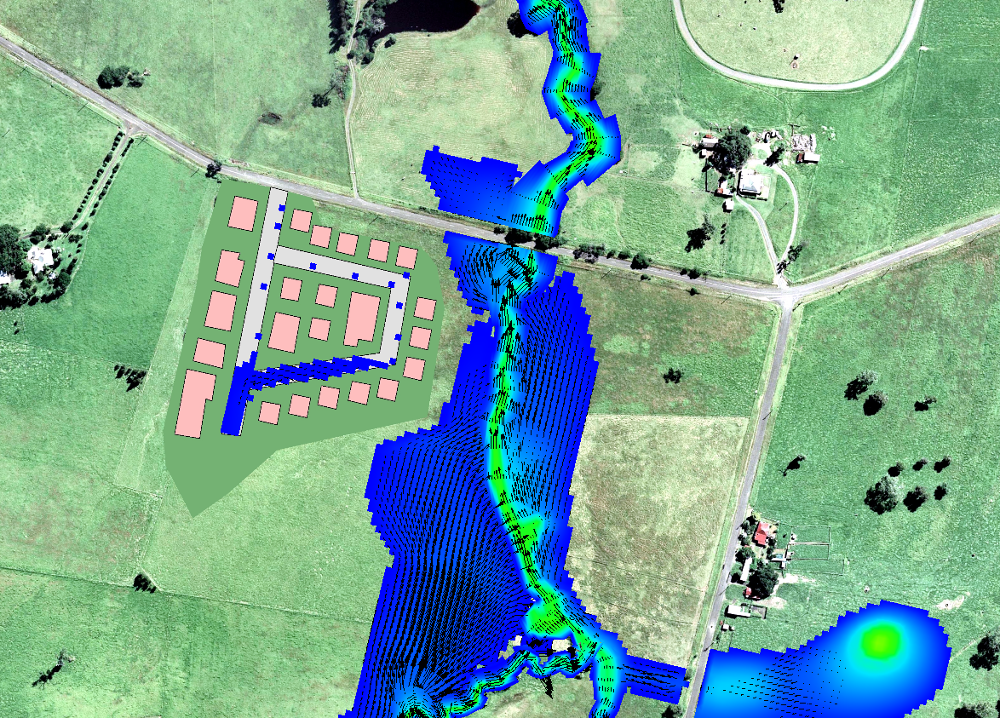
Open the 2D results in the TUFLOW results viewer. It can be seen that during the flood event the capacity of the pipe network is exceeded resulting in flooding of the roads in the proposed development.
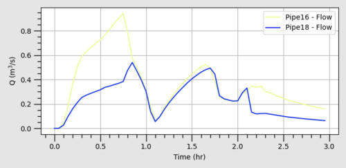
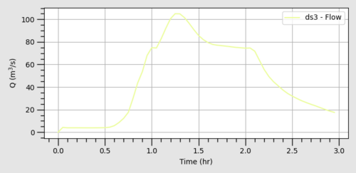
The 1D ESTRY results can be viewed by opening the time series results using the approach described in the following page: TUFLOW Viewer - Load Results - Time Series. You can also open results from Flood Modeller within the TUFLOW Viewer using the instructions here: TUFLOW Viewer - Load Results - Time Series FM
It can be seen that there is negative flow in Pipe16 and Pipe18 when the water levels in the Flood Modeller node and the connected ESTRY nodes are such that backwater effects are present.

A sense check of the flows being transferred across the "X1DQ" link can also be performed by plotting and comparing the flow time series for the first ESTRY node (ds3) and the last Flood Modeller node (ds2).

We have now completed the tutorial and you should now be familiar with the approaches of linking Estry to Flood Modeller and vice versa.
| Up |
|---|
