TUFLOW CATCH Tutorial M02 Results QGIS: Difference between revisions
| (38 intermediate revisions by the same user not shown) | |||
| Line 1: | Line 1: | ||
| ⚫ | |||
<font color="red"><font size=18>Page Under Construction</font></font> |
|||
Review how the intervention devices are removing pollutants using the TUFLOW CATCH interventions output summary and the TUFLOW HPC mesh results.<br> |
|||
| ⚫ | |||
Refer to <u>[[TUFLOW_CATCH_Tutorial_M01_Results_QGIS | TUFLOW CATCH Tutorial 01]]</u> for information on mass balance and boundary condition timeseries outputs. |
|||
Use the TUFLOW CATCH plugin to create a TUFLOW CATCH JSON file to review the TUFLOW HPC and TUFLOW FV results simultaneously. |
|||
== TUFLOW CATCH Interventions Output Summary == |
|||
==Create JSON File== |
|||
Review the interventions summary: |
|||
Create a TUFLOW CATCH JSON file: |
|||
<ol> |
<ol> |
||
| ⚫ | |||
<li> Go to Processing > Toolbox from the top drop down menu options to open the Processing Toolbox. |
|||
<li> This file contains final cumulative flows, masses entering and masses removed for all intervention devices and pollutants.<br> |
|||
<li> Go to TUFLOW Catch in the processing tool list and select <font color=red> create page?</font> <u>'Create TUFLOW Catch JSON'</u>. This opens the dialog shown below. |
|||
'''Note:''' The values in this results file may vary due to the spatial placement of intervention devices ('''2d_im_TC02_001_L''').<br> |
|||
* Results: Click '...', and select 'Add File(s)...'. Navigate to the '''Modelling\TUFLOWCatch\results''' folder and select '''TC02_001_catchment_hydraulic.xmdf''' and '''TC02_001_receiving_HD.nc''' (hold Ctrl to select multiple). |
|||
<br> |
|||
* Output File: Click '...', and navigate to the '''Modelling\TUFLOWCatch\results''' folder. Save the output file as '''TC02_001.tuflow.json'''. |
|||
[[File: TC2_interventions_summary_01a.png]]<br> |
|||
* res_to_res.exe: Click '...', and navigate to the '''TUFLOW_CATCH_Tutorial_Models\exe\res_to_res.2024-02-AA''' folder. Select '''res_to_res_w64.exe'''. |
|||
<br> |
|||
<li> Click 'Run'. Once the tool has finished, click 'Close'. |
|||
<li> Notice that bufferStrip1 has no pathogen masses entering or being removed, as it has no paddocks near it. |
|||
| ⚫ | |||
<li> If the removed mass is divided by the cumulative mass, the resulting value represents either the removal constant (if a constant removal equation was used), or the average removal performance (if a table removal method was used). For example, in trench1, the removal performance for SED_CLAY is calculated by: |
|||
<li> This will open up a 'Temporal Controller' dock. Hit F7, to open the 'Layer Styling' panel. The Temporal Controller dock and the Layer Styling panel will be used to review the simulation outputs. |
|||
<pre>rem SED_CLAY [g] / cum SED_CLAY [g] = 124003.900 / 310009.800 = 0.400 </pre> |
|||
This value (0.4) matches the removal constant. This constant was specified in the mass removal properties for pollutant 'SED_CLAY' for intervention device 'trench1' in the .tcc.<br> |
|||
In contrast, bufferStrip1 uses a table removal method for SED_CLAY, resulting in: |
|||
<pre>rem SED_CLAY [g] / cum SED_CLAY [g] = 283391.500 / 283590.600 = 0.999 </pre> |
|||
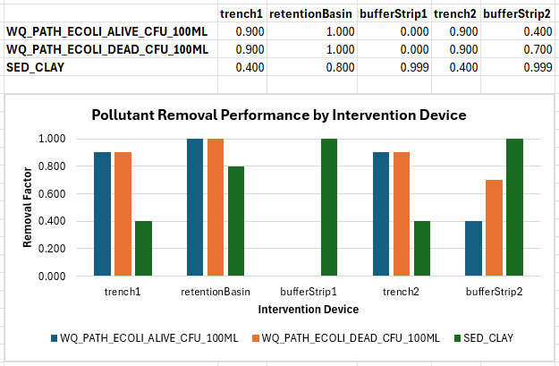
This shows that bufferStrip1 removed significantly more clay than trench1. The graph below demonstrates this calculation for each pollutant across all the treatment devices: <br> |
|||
<br> |
|||
[[File: TC2_removal_performance_all_devices_01a.png]]<br> |
|||
<br> |
<br> |
||
{{Video|name=}}<br> |
|||
</ol> |
</ol> |
||
==TUFLOW |
==TUFLOW HPC Map Outputs == |
||
Review the TUFLOW HPC Map outputs with the <u>[[TUFLOW_Viewer | TUFLOW Viewer]]</u>: |
|||
:'''Note:''' For further guidance on how to plot, view and style results, please refer to <u>[[TUFLOW_Viewer | TUFLOW Viewer]]</u>. |
|||
<ol> |
<ol> |
||
<li> Load the '''2d_im_TC02_001_L.shp''' layer from the '''TUFLOW\model\gis''' folder into QGIS. |
|||
<li> In the Layer Styling panel, go to the 'Datasets' tab. There is a list of all available output types. Select 'Depth'. |
|||
<li>Open TUFLOW Viewer from the TUFLOW Plugin toolbar.<br> |
|||
| ⚫ | |||
<li> In the Temporal Controller dock, use the time slider to view the depth results throughout the model simulation. |
|||
<br> |
<br> |
||
[[File:tuflow_plugin_tuflow_viewer.png]]<br> |
|||
{{Video|name=}}<br> |
|||
<li> In the Datasets tab, select 'Velocity' - both the contours [[File: image of contour button]] and the vectors [[File: image of vector button]]. |
|||
<li> In the Vectors tab, set 'Arrow Length' to 'Scaled to Magnitude'. |
|||
<li> Use the time slider to observe the water flowing from the catchment area into the TUFLOW FV model domain. |
|||
<br> |
<br> |
||
<li>Open TUFLOW Viewer from the TUFLOW Plugin toolbar and open the simulation results. Select File > Load Results - Map Outputs. Navigate to the '''TUFLOWCATCH\results''' folder and select '''TC02_001_catchment_hydraulic.xmdf'''. |
|||
{{Video|name=}}<br> |
|||
<li> In the TUFLOW Viewer panel, select 'Conc WQ_PATH_ECOLI_ALIVE_100ML' from the Result Type list. Adjust the symbology as needed. Refer to <u>[[TUFLOW_CATCH_Tutorial_M01_Results_QGIS#TUFLOW_HPC_Map_Results | TUFLOW CATCH Tutorial 01]]</u> for details. |
|||
<li>Use the time slider to view the pathogen concentration results. Notice how the E. coli is removed by the treatment devices. In areas where there are no interventions, the pollutant concentrations are much higher (i.e. the eastern waterhole).<br> |
|||
<br> |
|||
{{Video|name=animation_TC2_results_01a.mp4|width=1432}}<br> |
|||
| ⚫ | |||
<li>Zoom in to bufferStrip1. Use the Plot Time Series tool (from Map Multi) to place a timeseries point on either side of the intervention device to see how bufferStrip1 is removing the sediment.<br> |
|||
<br> |
|||
{{Video|name=animation_TC2_results_02a.mp4|width=1432}}<br> |
|||
<li>Using the same process as above, observe the mass removal occurring at the other intervention devices. <br> |
|||
<br> |
|||
{{Video|name=animation_TC2_results_03a.mp4|width=1432}}<br> |
|||
</ol> |
</ol> |
||
<br> |
<br> |
||
{{Tips Navigation |
{{Tips Navigation |
||
|uplink=[[TUFLOW_CATCH_Tutorial_M02#Check_Files_and_Results_Output| Back to TUFLOW CATCH Tutorial |
|uplink=[[TUFLOW_CATCH_Tutorial_M02#Check_Files_and_Results_Output| Back to TUFLOW CATCH Tutorial 02]] |
||
}} |
}} |
||
<br> |
|||
Latest revision as of 15:22, 9 July 2025
Introduction
Review how the intervention devices are removing pollutants using the TUFLOW CATCH interventions output summary and the TUFLOW HPC mesh results.
Refer to TUFLOW CATCH Tutorial 01 for information on mass balance and boundary condition timeseries outputs.
TUFLOW CATCH Interventions Output Summary
Review the interventions summary:
- In Windows File Explorer, navigate to the TUFLOWCATCH\results folder and open TC02_001_catchment_hydraulic_intervention_summary.csv.
- This file contains final cumulative flows, masses entering and masses removed for all intervention devices and pollutants.
Note: The values in this results file may vary due to the spatial placement of intervention devices (2d_im_TC02_001_L).
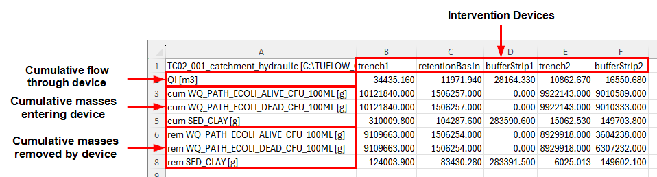
- Notice that bufferStrip1 has no pathogen masses entering or being removed, as it has no paddocks near it.
- If the removed mass is divided by the cumulative mass, the resulting value represents either the removal constant (if a constant removal equation was used), or the average removal performance (if a table removal method was used). For example, in trench1, the removal performance for SED_CLAY is calculated by:
rem SED_CLAY [g] / cum SED_CLAY [g] = 124003.900 / 310009.800 = 0.400
This value (0.4) matches the removal constant. This constant was specified in the mass removal properties for pollutant 'SED_CLAY' for intervention device 'trench1' in the .tcc.
In contrast, bufferStrip1 uses a table removal method for SED_CLAY, resulting in:rem SED_CLAY [g] / cum SED_CLAY [g] = 283391.500 / 283590.600 = 0.999
This shows that bufferStrip1 removed significantly more clay than trench1. The graph below demonstrates this calculation for each pollutant across all the treatment devices:


TUFLOW HPC Map Outputs
Review the TUFLOW HPC Map outputs with the TUFLOW Viewer:
- Note: For further guidance on how to plot, view and style results, please refer to TUFLOW Viewer.
- Load the 2d_im_TC02_001_L.shp layer from the TUFLOW\model\gis folder into QGIS.
- Open TUFLOW Viewer from the TUFLOW Plugin toolbar.
- Open TUFLOW Viewer from the TUFLOW Plugin toolbar and open the simulation results. Select File > Load Results - Map Outputs. Navigate to the TUFLOWCATCH\results folder and select TC02_001_catchment_hydraulic.xmdf.
- In the TUFLOW Viewer panel, select 'Conc WQ_PATH_ECOLI_ALIVE_100ML' from the Result Type list. Adjust the symbology as needed. Refer to TUFLOW CATCH Tutorial 01 for details.
- Use the time slider to view the pathogen concentration results. Notice how the E. coli is removed by the treatment devices. In areas where there are no interventions, the pollutant concentrations are much higher (i.e. the eastern waterhole).
- Select 'Conc SED_CLAY' from the Result Type list. Adjust the symbology as needed.
- Zoom in to bufferStrip1. Use the Plot Time Series tool (from Map Multi) to place a timeseries point on either side of the intervention device to see how bufferStrip1 is removing the sediment.
- Using the same process as above, observe the mass removal occurring at the other intervention devices.

| Up |
|---|