FMA Challenge 1 (1D-2D linked)
Introduction
The FMA Challenge series provide example projects for intermediate to advanced TUFLOW users. If you are just starting out or haven't already completed the tutorial models, please see this tutorial model page.
In this challenge, a fully two-dimensional model with a nested one dimensional model has been developed to explore in and over-bank floodplain conditions. The model includes several hydraulic structures/bridges within the main stream system which impact flood elevations. Flooding of the urbanised over-bank floodplain is expected.
A fully functional example model has been developed by BMT WBM, allowing you to review the model setup, run the model and review results developing your skills in:
- Nested 1D/2D models;
- Understanding urban riverine conditions and over-bank floodplains;
- Understanding the impact of data quality on DEM development;
- Understanding of the influence of hydraulic structures;
- Using scenarios and variables to determine a suitable cell size, timestep and log output scenarios; and
- Using bc layers with HX, XP, CD and CN types.
Data for this model is provided via ZIP compressed file posted on the internet/FTP WHERE IS THIS??? for download.
Relevant Tutorials
Although all Tutorials are of relevance for the FMA Challanges, For FMA Challange 1, it may be useful to revisit the following:
- 1D-2D Linking- Tutorial Module 2
- Running Events and Scenarios- http://www.tuflow.com/forum/index.php?showtopic=1149&hl=scenario
Model Setup
This section details the setup of the fully functional model developed by BMT WBM. All files required to re-run the model can be found at FMA_Challenge_Models/FMA_Scenario1/. It is at your discretion which GIS package, text editor and method of model simulation to use (batch mode or within the text editor).
Cross Section Spacing, Grid Size and Mesh Element Size
1D sections were used for the in-bank topography. The overbank (2D) areas were modelled using 10ft and 15ft resolutions. The 2D grid dimension (rotated) was 17,500ft by 8,000ft. A total of 87 cross-sections were used for the 1D in-bank domain.
Structures were modelled as a combination of bridges and culverts. For bridges, height varying energy loss tables were used based on the Hydraulics of Bridge Waterways (Bradley, 1978). For culverts, TUFLOW simulates all possible inlet and outlet controlled flow regimes with automatic switching between regimes. The calculations of culvert flow and losses are carried out using techniques from “Hydraulic Charts for the Selection of Highway Culverts” and “Capacity Charts for the Hydraulic Design of Highway Culverts”, together with additional information provided in the literature such as Henderson 1966.
The number of cross sections and mesh elements used are as follows:
| 2D Cell Size | 1D Sections | Active 2D Cells |
|---|---|---|
| 15ft | 50 | 286,434 |
| 10ft | 87 | 643,565 |
Computational Domain Assembly
TUFLOW directly reads GIS data layers to construct models. The layers used/created for Challenge 1 are:
- A DEM TIN created from the provided terrain data (2ft contours) and exported to ESRI ASCII format as a 2ft DEM grid. When TUFLOW reads this DEM it interpolates the elevations onto the 2D computation grid.
- GIS layers of cross-section locations and 1D network including structure details.
- GIS land-use layer digitized in .shp format.
- GIS layer of 1D/2D interface lines along the left and right banks of the channels.
All model inputs are independent of the 2D grid cell size, orientation and extent, allowing for different 2D resolutions, dimensions and orientation to be easily simulated. Peak flood depths and water levels were exported to ESRI ASCII grids, and the flood extent was created by contouring the grid into a single region. Flows are outputted in .csv format and directly loaded into Excel. Profiles were created using the post processing utility TUFLOW_to_GIS and outputted into a .csv file.2D Grid Resolution
A 15ft 2D grid resolution is extensively used for urban modeling, and in this case provides a good trade-off between resolution and run time. 15ft cells are small enough that flow paths down roads are adequately represented (provided the DEM accurately represents the roads as discussed above).
To test the effect of different resolutions, simulations were made using grid resolutions of 5, 10, 15, 20 and 40 ft. Upon examination of the results, the flood extents varied by unexpected amounts between different resolutions. For example, the 10ft grid scenario (provided as part of the ftp download) produces a more extensive flood extent, even though the profile down the 1D channel is almost identical to the 15ft case. The extended flooding is the result of very shallow flow (less than 0.01ft deep) over large flat (horizontal) areas caused by the use of contours to create the DEM as discussed above. Due to the slightly coarser resolution the 15ft grid does not let water on to some of these flats, and they remain dry. Should an accurate DEM be made available for this Challenge, the flood extents are likely to be very different and much more consistent between different grid resolutions!
This does raise one issue indirectly of flood mapping in urban areas where the flood depths are very shallow, or if using direct rainfall modeling. In these instances, mapping of urban areas may specify that flooding must be of a minimum depth to be mapped. For example, where the flooding is less than say, 0.05m, it is not mapped.
Manning's n Values
The Manning’s n values were based on the aerial photo and structure photos as tabulated below. A sensitivity simulation was carried out increasing the Manning’s n value along the main channel from 0.03 to 0.04. The results for the sensitivity simulation are provided in the long-profile of maximum water surfaces along the channel (depth grids and other data can be provided upon request). The maximum increase in peak water level along the profile is 1.94 ft.
Land Use Manning's n Main Channel 0.03 Roads 0.02 Properties (Buildings, Gardens and Fences) 0.1 Crop 0.05 Parkland 0.035 Vegetated area adjacent creek 0.06 Pasture 0.045 Challenges
The typical challenges experienced in situations similar to this usually relate to:
- The use of contour data to create the DEM; and
- The model boundary/terrain data does not extend beyond the flooded area.
The presented solutions to these challenges are as follows:
Using Contour Data to Create the DEM
Contour data, without additional point elevations and/or 3D breaklines, is difficult to triangulate or interpolate to create an accurate DEM. The consequence of solely using contours is the resulting DEM can have a terraced or stair-step surface that contains flat sections where the contours form a U shape.
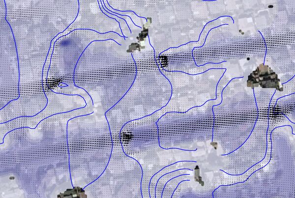
For example, the image below shows a part of the DEM. The red lines are the 2ft contours provided. Where the contours form a U shape, the triangulation or interpolation method typically forms flat (horizontal) areas inside the U as labeled “Flat” in the image. Between the Flats, Steps occur representing the drop in elevation to the next contour level.

When the 2D flow patterns are observed, as per the velocity arrows in the image below, the water appears to be “cascading” down the roads. Along the flat areas the velocities are low, and where the elevations suddenly drop to the next flat section the velocities are high, thereby creating the cascading effect.
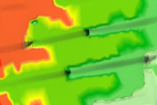
The 2D flow patterns reflect the terraced or stepped nature of the DEM, which is not a realistic representation of the road topography. Some interpolation methods such as IDW (Inverse Distance Weighting) can provide a smoother DEM, but may not preserve the contours, and where the U shapes are pronounced they will still have a strongly terraced effect.The resulting 2D depths and water levels are also unrealistic as can be seen in the image below. The blue shades are the depths and the blue lines the water level contours every 0.5ft. Where the steps occur in the DEM, the water level contours are closely spaced, and along the flats they are wide apart. The depths vary significantly along the road when they should be reasonably uniform.
For 2D modeling, especially in flat urban areas, contours should not be used to create the DEM. If the contours were generated from a DEM, then the original DEM should be used or the original terrain data should be provided and the DEM recreated from this data. If contours are used, additional point data and/or 3D breaklines along the low and high points need to be provided to prevent the terraced effect from occurring.
The Model Boundary and Terrain Extent
The flooding in the overbank 2D domain extends to the edge of the model boundary and terrain data. The terrain data needs to be extended further afield to high ground.
Conclusion
We have explored an Urban Riverine conditions with an urbanized over-bank floodplain. Now we have a better grasp of nested 1D/2D models, influence of hydraulic structures, use of scenarios and variables to determine cell sizes, timesteps and log outputs, and using bc layers with HX, XP, CD and CN types in synergy.
Congratulations on finishing Challenge 1!


