Difference between revisions of "TuPlot"
| Line 125: | Line 125: | ||
[[File:TuPlot LongProfile 03.PNG]] | [[File:TuPlot LongProfile 03.PNG]] | ||
| − | =Plotting 1d_ta (tabular data)= | + | ==Plotting 1d_ta (tabular data)== |
| + | To plot 1d tabular data (1d cross sections, 1d losses, 1D nodal area), the step in TuPlot are: | ||
| + | * Open the relevant 1d_xs or 1d_ta GIS layer. This should be in the format outlined in the TUFLOW manual. | ||
| + | * Select feature(s) to plot | ||
| + | This workflow is shown in the image below.<br> | ||
| + | [[File:TuPlot TabularData 01A.PNG]] | ||
| + | <br> | ||
| + | If the cross-section has roughness data (the '''Flags''' attribute includes '''M''' [material ID] or '''n''' [Manning's n]) this can be visualised by navigating to the options tab and checking the box for '''Display Roughness''' (see [[TuPlot#TuPlot_Window | TuPlot window]] above. An example is shown in the image below.<br> | ||
| + | |||
| + | [[File:TuPlot TabularData 02.PNG]] | ||
Revision as of 18:19, 22 March 2016
THIS PAGE IS PRESENTLY BEING UPGRADED
Introduction
The TuPlot functionality is a python based tool for plotting inputs and output from TUFLOW. For the 2016 version of TUFLOW a new output format was made available, this has the following changes from previous versions:
- Combines the 1D results, 2D plot outputs and new reporting location data
- The outputs are stored in a separate Plot folder in the TUFLOW results directory
- .tpc (TUFLOW Plot Control file links to data in csv and gis folders
- Has additional Node and Channel information files contain connectivity information
This is the default approach for the 2016 version but can be modified with the TUFLOW command "Output Approach == Pre 2016" (refer to the manual for more information on this command.
The TuPlot utility is currently available as part of a QGIS plugin, however, future plans include extending this to ArcMap and as a standalone viewer.
TUFLOW Python Results Library
The TuPlot plotting utility relies on a python library TUFLOW_results2016.py for loading the TUFLOW results. This python based library can also be used to access TUFLOW results from python (outside of TuPlot). Please refer to python TUFLOW results library for more information and examples of this.
QGIS TuPlot
This plotting functionality is currently accessed via QGIS. Ensure that the QGIS plugin is installed via the instructions on the TUFLOW QGIS plugin page.
Once this has been installed successfully QGIS can be open and the plugin accessed via the Plugin >> TUFLOW >> TuPlot menu item, or via the TuPlot button in the toolbar. The toolbar icon is shown below.
TuPlot Window
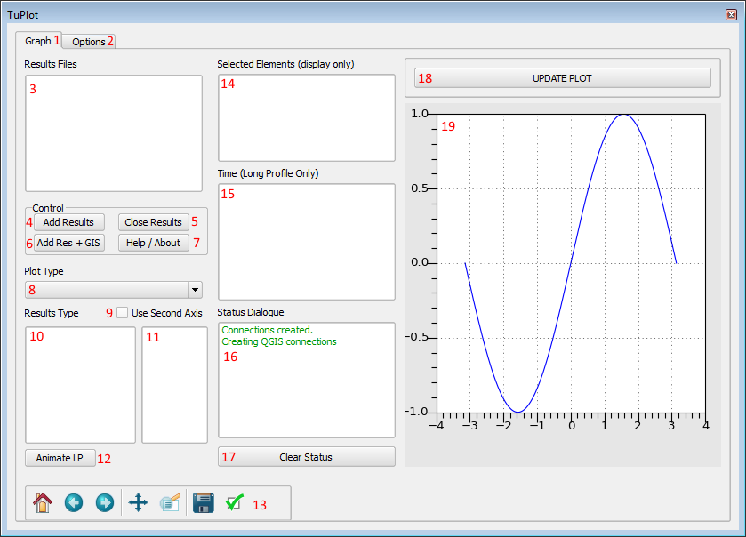
Once the plot viewer has been opened a plot window as per the below images will be opened. The features have been numbered in the images below and a description of each is provided below.
This window in QGIS is re-sizeable and dockable, you can:
- un-docked to allow this window to moved to a second monitor
- move the position of the window to a different location, e.g. below the map window
- resized as desired
Graphing Window of TuPlot
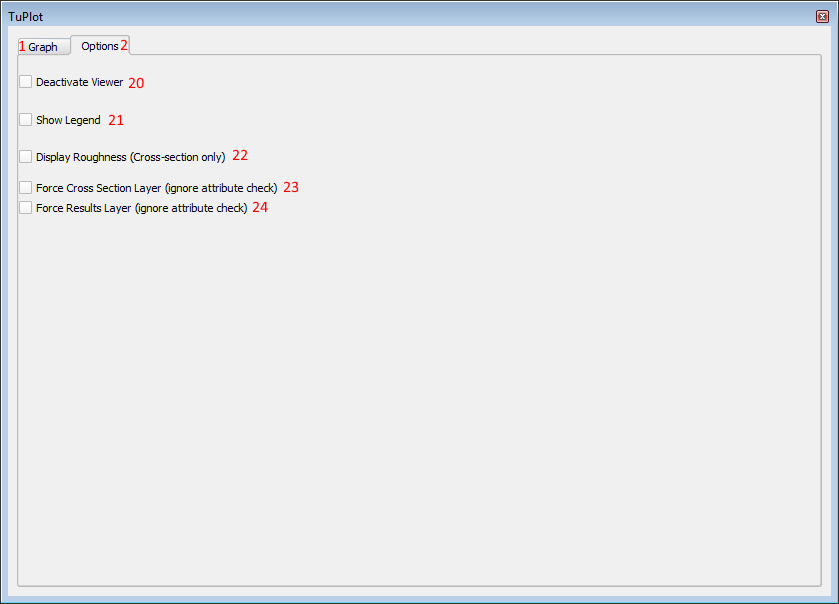
Options Window of TuPlot
The features on each of the windows is described below, with the number corresponding to the numbers in the two images above.
- Switch to the Graph tab of TuPlot, this is the default view
- Switch to the Option tab of TuPlot
- A list of the currently open results files
- Add results only (no GIS layers), see Loading Results below for more information
- Close results file selected in the results file list (3)
- Add results and relevant GIS layers, see Loading Results below for more information
- Opens an about dialogue. Also contains a link to this page
- Allows the user to switch between time-series and long profile plotting, see below for more information on plotting time-series and long profiles
- Check box to enable dual y axis plot
- List of available results types to be plotted on the primary Y axis
- List of available results types to be plotted on the secondary axis
- Animate LP. Start an animation of the Long Profile data. There must be data loaded and the Plot Type (8) above should be set to Long Profile
- matplotlib toolbar - this contains options for changing the zoom and customising the plot window.
- Selected elements view. This contains a list of the ID's of the selected elements (1D, 2D or RL). This is for display only. Changing the selection here does not alter the plot
- Time step selection. This is only valid for Long Profile viewing, see Long Profiles below
- Status dialogue. This contains information on the status of the TuPlot utility. If there are any warnings or errors these should be displayed in the status window.
- Clear Status. This can be used to clear previous messages to the status dialogue
- Update plot, if the options or results types have been modified, this button can be used to redraw the plot window
- This is the plot window containing the time-series, long profile or cross-section plot The following features are available in the Options tab. After changing any of these settings, you will need to select the update Plot or change the selection in the QGIS map window to force a re-draw of the plot window.
- Deactivate viewer can be used to temporarily disable the TuPlot window, so that changing the selection, active layer will not cause the plot window to update
- Show legend - toggle the legend on or off for the plot. The default is off
- Display Roughness - this is only valid for viewing cross-sectional data. If the cross-section has varying roughness (M or N flag specified on the section) this will display the roughness information on a secondary y axis
- Force Cross-section layer. When a TUFLOW cross-section layer is input into TUFLOW, it has the attributes Source, Type, Flags, Column_1, Column_2 etc. When the TuPlot utility encounters a map layer, it searches for these attribute names to determine if the layer is a 1d_tab or 1d_xs layer. If it is not, plotting for the layer is disabled. By enabling this check box, the checking of the layer attributes is suppressed. This will attempt to plot the data regardless of the attributes, however, if the data is not a valid 1d_tab format this may cause issues / errors with the plotting. For example if the 1st attribute is not a source .csv file, the utility will be unable to open this and read the content.
- Force Results Layer. When determining if the GIS file selected in the layer control is a TUFLOW output file, TUFLOW checks that the attribute names match the output format from TUFLOW. Each of the GIS layers referred to in the .tpc file has three attributes: ID, Type and Source. By enabling this check box, the checking of the layer attributes is suppressed. This will attempt to plot the data regardless of the attributes, however, if the data is not in valid format this could cause issues with TuPlot.
Loading Results
In order to be able to visualise the results these results need to be loaded into the Plugin. This can be done with the Add Results or Add Res + GIS buttons. The difference between these is:
- Add Res + GIS will load all the .csv file data into memory and also add the GIS layers to the current QGIS project. These are defined in the .tpc as:
- GIS Plot Layer Point == .\gis\<filename>_PLOT_P
- GIS Plot Layer Lines == .\gis\<filename>_PLOT_L
- GIS Plot Layer Point == .\gis\<filename>_PLOT_P
This is the preferred approach for reading in a single results file.
- Add Results will only load in the .csv files and not the GIS data. This can be used if a set of results is already open to avoid duplication of GIS layers in the project.
After a set of results, with GIS files has been loaded, the QGIS window will look like the below:
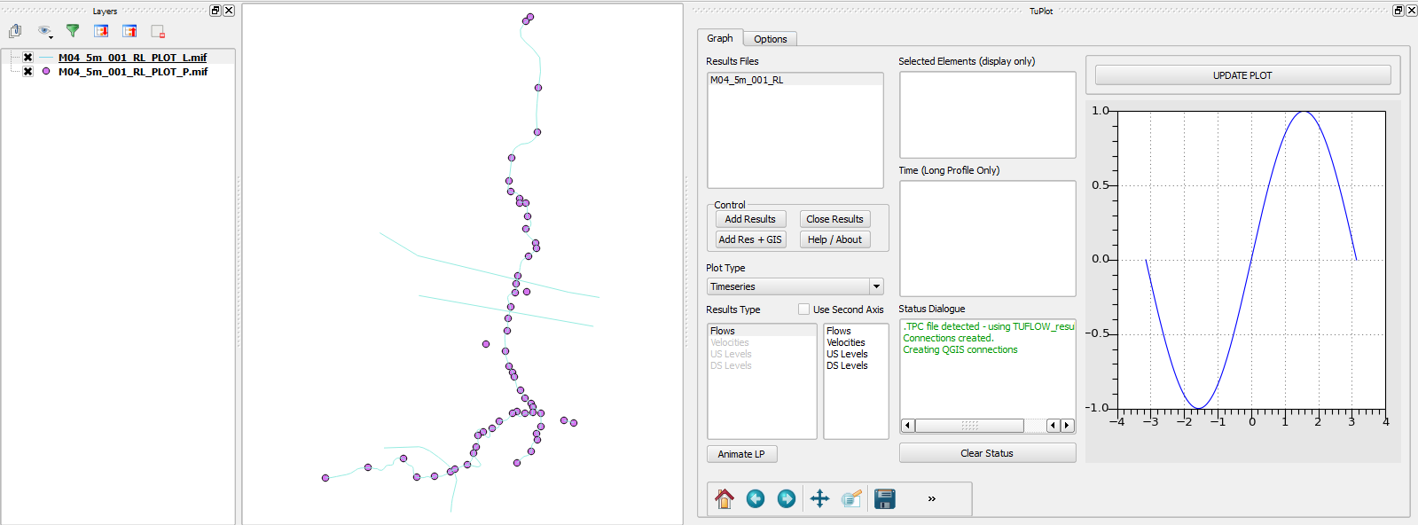
The layer window shows that two GIS layers have been loaded, these contains points (1D nodes, 2D plot output and reporting location points) and lines (1D channels, 2D plot output and reporting location lines).
Time-series
The default plot type for viewing results is Timeseries. Once results have been loaded (as per the above), select the GIS layer to plot from, the points and the lines contain different data:
The _P (points) contains 1D node and 2D plot output / reporting location point data. This is typically water or energy level, depending on the output setting for the simulation.
The _L (lines) contains 1D channels, 2D plot output and reporting location lines. This may include flows, velocities and flow areas depending on the output setting for the simulation.
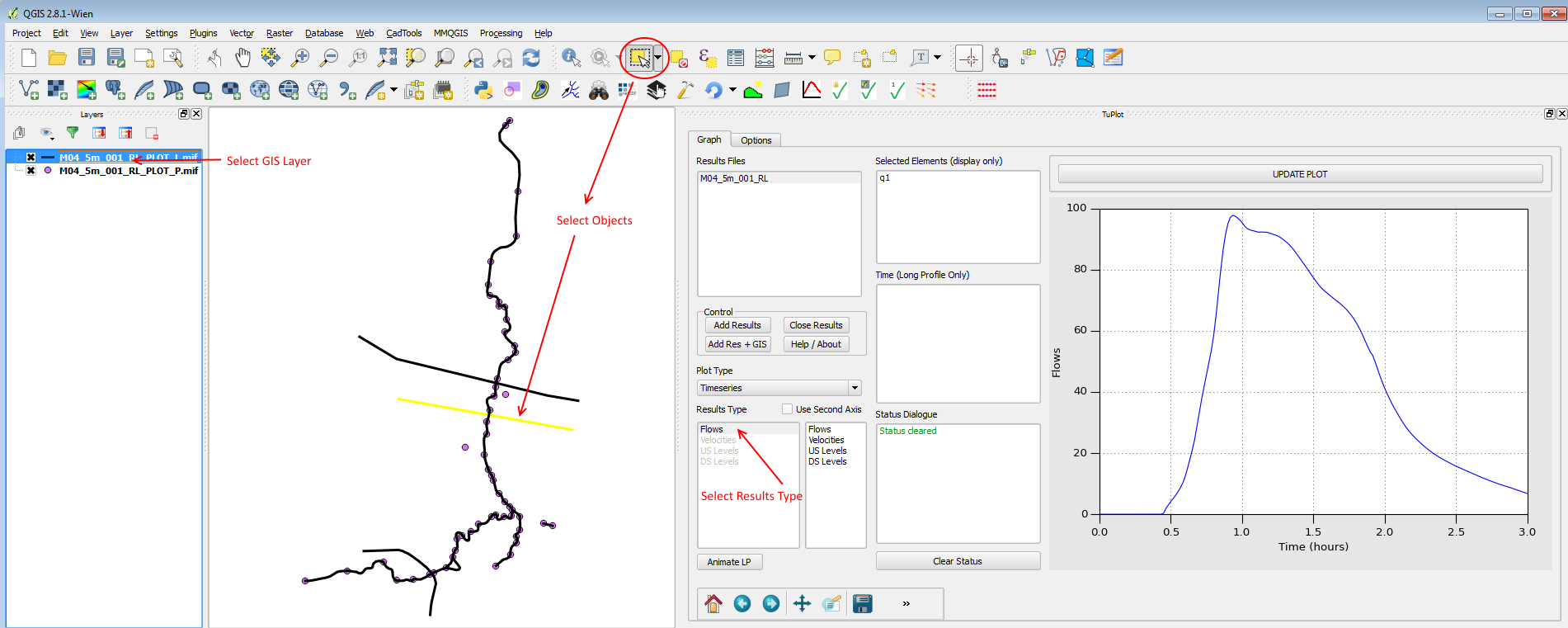
Once a GIS layer has been chosen, the Select Features tool can be used to select features in the map window. Multiple features can be selected by holding the 'control' key and click again, or by dragging a rectangle around multiple features.
Once a feature(s) has been selected, the data will be plotted. The results types list can be used to select the type of data. Multiple results types can be selected.
The annotated image below, shows the workflow.
Dual Axis
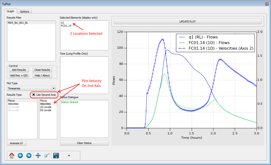
A secondary y-axis is available to plot data. For example flows and velocities are likely to have quite different ranges. In the image below, two GIS locations are selected:
- q1 is a reporting location which sums the flows from the main channel as well as over-bank areas. This RL only has flow data available and not velocity data.
- FC01.14 is a 1D channel and has both flow and velocity results available.
In the case below the 2nd axis is enabled with the highlighted check box, and the data to be plotted on the secondary axis is velocity. The primary data is the flow data. The legend has been enabled in the Options tab.
Three lines are plotted in the image below, flows for both the reporting location and channel and velocities only for the 1D channel.
Multiple Results Files
Multiple results files can be opened, see Loading Results above.
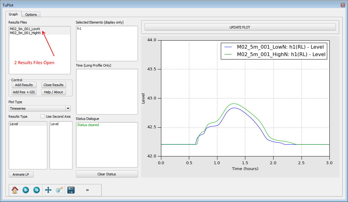
In the image two results files have been opened (the 1st using Add Res + GIS and the second with the Add Results button. These are:
- M02_5m_001_LowN - A low Manning's n case of Tutorial Module 2 with Manning's decreased by 20% with the .tcf command "Read Materials File == ..\model\materials.csv | 0.8 !Decrease Roughness by 20%"
- M02_5m_001_HighN - A high Manning's n case of Tutorial Module 2 with Manning's increased by 20% with the .tcf command "Read Materials File == ..\model\materials.csv | 1.2 !Increase Roughness by 20%"
With both sets of results loaded a reporting location has been used to plot the water levels for both the low and high Manning's n scenarios. As expected the higher Manning's n results in an increased water level.
Long Profiles
Long profiles can be plotted using the TuPlot utility for 1D sections only. When dealing with 1D long profile data, if a single 1D channel is specified the data for all channels downstream will be plotted. If two channels are specified, long profile data will only be returned for the channels between the specified channels (an error occurs if the channels are not connected). If more than 2 channels are selected, a warning is given and only the 1st two channels are used.
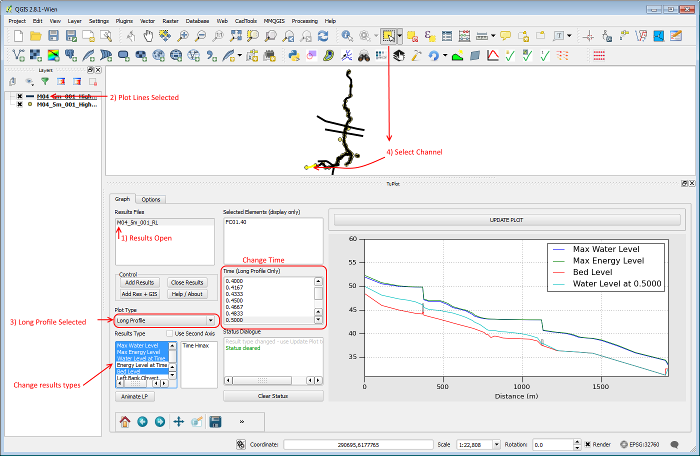
To plot a long profile, the steps are:
- Ensure that a results file is open
- Ensure that that plot lines are selected in the layer control
- Select Long Profile in the Plot Type dropbox.
- Select one or two 1D channels.
This workflow is outlined in the image below.
Once a profile has been created (or before) the user can select the type of results to be plotted in the Results Type list. In the plot above the plotted results are, maximum water level, maximum energy level, water level at time and bed level. If this is changed the Update Plot will need to be selected to redraw the plot, or the selection in the can be changed as this will trigger a re-draw.
If plotting a water level or energy level at a time, the Time list can be used to change the currently plotted time. When this is changed the plot is automatically re-drawn.
Adverse Gradients
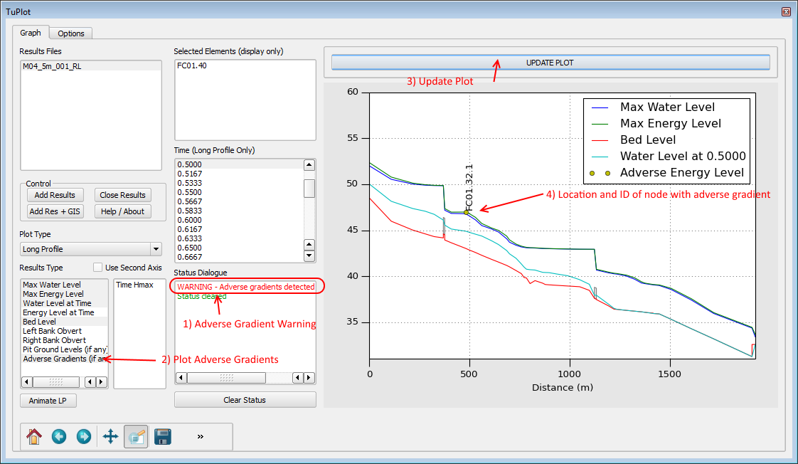
When TuPlot determines the channels to be plotted, a check is performed that the water levels or energy levels (if they have been output) decrease as you go downstream. If there are adverse gradients detected TuPlot will issue a warning in the Status Dialogue.
It could be that an adverse gradient is normal, i.e. a storm surge into a drainage channel. However, it could also indicate that a channel is digitised incorrectly or that an instability has occurred.
The Adverse gradient results type can be enabled to see where on the long profile these occur, and if the legend is turned on the 1D node ID's. This can be seen in the image below.
Animate Long Profile
The TuPlot utility can save out a series of images (in the .png format) of each of the timesteps in the long profile data. These are saved out to the .tpc folder and are given a sequential number. These can be converted into a video using software such as Windows movie maker or ffmpeg. Future versions of TuPlot will look to create the animations from the images automatically.

Plotting 1d_ta (tabular data)
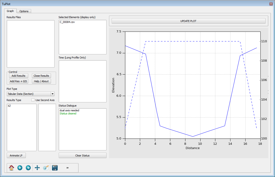
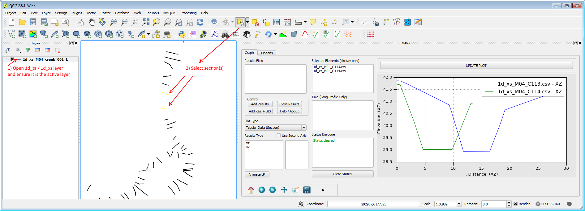
To plot 1d tabular data (1d cross sections, 1d losses, 1D nodal area), the step in TuPlot are:
- Open the relevant 1d_xs or 1d_ta GIS layer. This should be in the format outlined in the TUFLOW manual.
- Select feature(s) to plot
This workflow is shown in the image below.
If the cross-section has roughness data (the Flags attribute includes M [material ID] or n [Manning's n]) this can be visualised by navigating to the options tab and checking the box for Display Roughness (see TuPlot window above. An example is shown in the image below.
