Flood Modeller Tutorial Module01 Provisional
Introduction
In this module, an existing 2D TUFLOW domain is linked to a Flood Modeller 1D model.
The 2D domain represents the floodplain, while the 1D model represents the watercourse and in-channel structures. Linked 1D–2D models combine the strengths of both approaches. Here, the 1D scheme represents the largely unidirectional flow of the watercourse, while the 2D scheme captures the more complex floodplain hydraulics.
In the below 2D model example, the main channel is only 5-10 m wide, making the 5 m grid resolution too coarse to represent it accurately. This reduces the accuracy of conveyance within the channel.

There are several options for improving the representation of this creek channel:
- Decrease the width of the 2D cells, either globally or by using Quadtree, and/or apply sub-grid sampling.
- Model the channel as a 1D network dynamically linked to the 2D domain (the floodplain).
For this module, the second option will be demonstrated.
TUFLOW can also link with other 1D solvers, including ESTRY (TUFLOW 1D), XP-SWMM and 12D Solutions’ Dynamic Drainage. Setting up a channel that cuts through a 2D domain is typically one of the more time-consuming modelling tasks.
For this module, the complete Flood Modeller 1D model network has been provided, to allow for progressing through the module in a relatively short period of time.
Linking Flood Modeller to TUFLOW
It is assumed from the outset of this module that Flood Modeller has already been linked to the desired version of TUFLOW. There are four methods by which Flood Modeller and TUFLOW can be linked, all of which are described on this page.
Using the Flood Modeller interface to set the location of the TUFLOW engine files for the TUFLOW build you want to use, is the simplest approach to linking Flood Modeller and TUFLOW and does not duplicate files. This method is recommended if it is expected that the same versions of Flood Modeller and TUFLOW will be used consistently when running linked models.
1) Open the Flood Modeller software and in the 'Home' tab select the 'General' option.

2) Select the 'Project Settings' sub-menu and within the TUFLOW Engine File Location choose to browse to the version of TUFLOW that you would like to link Flood Modeller to. Choose 'Open' and then 'OK'. It is recommended that the option 'Show Solver Window when Running Simulations' be switched on as well.

3) Save the changes that you have made to the setup. This will update the settings file (formed.ini).
4) Restart Flood Modeller to effect the revised setting.
4) The linked model can then be run by opening the .ief file within the Flood Modeller Interface and clicking Run.
Existing Model Data
This tutorial builds upon the 2D TUFLOW domain that was constructed as part of Module 1 and Module 2 of the TUFLOW Tutorial Model.
The model developed in these tutorial modules already contains some culverts modelled as 1D elements. The culverts are modelled in ESTRY, TUFLOW's internal 1D engine. One of these culverts will be kept in ESTRY and the other will be added to the Flood Modeller model. The 2D boundary conditions (upstream inflows and downstream stage-discharge boundary) will be removed from the model. These will instead be represented in Flood Modeller as it is a more typical schematisation for a 1D/2D linked model.
The existing TUFLOW model consists of:
- Definition of Active/Inactive Areas
- Definition of Land Use areas for the spatial distribution of roughness values
- 1D ESTRY culverts
- 1D/2D boundary links to connect the 1D ESTRY culverts to the 2D TUFLOW domain.
Project Initialisation
TUFLOW models are separated into a series of folders which contain the input and output files. The recommended set up for the model directory and sub-folders is shown below. For a more detailed description, refer to the [1].

| Sub-Folder | Input / Output | Description |
|---|---|---|
| bc_dbase | Input | Boundary condition database(s) and input time-series data. |
| check | Output | GIS and other check files to carry out quality control checks (use Write Check Files). |
| model | Input | Geometry (TGC), Boundary (TBC) and other model control text files (i.e. no GIS files). |
| model\gis | Input | GIS layers that are inputs to the 2D and 1D model domains are contained within this folder, model\gis is typically used for all QGIS and ArcGIS files. |
| model\mi | Input | GIS layers that are inputs to the 2D and 1D model domains are contained within this folder, model\mi is typically used for MapInfo formatted GIS files. |
| results | Output | TUFLOW outputs the results to this folder in specified formats. |
| runs | Input | TUFLOW Control Files (TCF). |
| runs\log | Output | TUFLOW log files (TLF) and messages layers. |
The TUFLOW folders can be set up manually, automatically running TUFLOW model with Write Empty GIS Files command or automatically through GIS programs:
- QGIS - SHP
- QGIS - GPKG
- SMS - the folder structure listed above is automatically created before running the model using the 'Export TUFLOW files' command (see Run TUFLOW from within SMS).
- ArcMap (10.1 and newer) - the ArcTUFLOW Toolbox can be used to automatically create the model folders, model projection, TUFLOW control files and run TUFLOW to create the template files.
The following points on TUFLOW folders and filenames are worth noting:
- TUFLOW accepts any folder structure, though the above listed format is most commonly used and is recommended.
- TUFLOW accepts spaces and special characters (such as ! or #) in filenames and paths, but other software may not. It is recommended that spaces and other special characters are not used in the simulation path and filenames.
- Folder paths, filenames, file extensions and TUFLOW commands are not case sensitive in any TUFLOW control files.
- Any directories that don't apply can be omitted, for example, if using QGIS or ArcMap the model\mi directory is not required.
- TUFLOW accepts any folder structure, though the above listed format is most commonly used and is recommended.
Model Familiarisation
Become familiar with the model location, using an aerial image and DEM:
GIS and Model Inputs
The steps required to modify each of the GIS inputs are demonstrated in QGIS using SHP and GPKG formats. Instructions for completing the module in ArcGIS or MapInfo are available on the archive page for Tutorial Module 01.
Define the External 1D Networks
This part of the module creates the GIS layers that specify the location of the Flood Modeller nodes that are to be connected to the 2D domain.
Follow the instructions below for the preferred GIS format.
Define the Water Level Lines
This part of the module creates the Water Level Lines that will be used to visualise 1D results in 2D map outputs.
Follow the instructions below for the preferred GIS format.
Define the 1D/2D Boundary Links
This part of the module creates the 1D/2D boundaries to link the Flood Modeller 1D component to the TUFLOW 2D domain.
Follow the instructions below for the preferred GIS format.
Define Bank Elevations
This part of the module defines the bank elevations of the watercourse which are the elevations of the 1D/2D boundary links created in the previous section.
Follow the instructions below for the preferred GIS format.
Deactivate 2D cells
This part of the module describes the steps to deactivate the 2D cells where the 1D model is replacing the 2D solution.
Follow the instructions below for the preferred GIS format.
Modify Simulation Control Files
With the input GIS layers modified, the next step is to update the TUFLOW control files and Flood Modeller simulation files to create a linked model.
TUFLOW Geometry Control File (TGC)
At this stage, the following changes will be made to the geometry:
- The cells along the watercourse that are represented in the 1D Flood Modeller component of the model are deactivated.
- Bank elevations along the watercourse are enforced.
- In the FMT_Tutorial\FMT_M01\TUFLOW\model folder, save a copy of M01_5m_002.tgc as FMT_M01_001.tgc.
- Open FMT_M01_001.tgc
QGIS - SHP
Add an extra command line after Read GIS Code ==..\model\gis\2d_code_FMT_M01_001_R.shp
Read GIS Code BC == gis\2d_bc_FMT_M01_HX_001_R.shp ! Deactivates the cells where the watercourse has been modelled in 1D
Note that the order of the commands is important. The layer 2d_code_FMT_M01_001_R.shp first activates cells within the modelled area, then the layer 2d_bc_FMT_M01_HX_001_R.shp deactivates selected cells along the watercourse.
QGIS - GPKG
Add an extra command line after Read GIS Code == 2d_code_FMT_M01_001_R
Read GIS Code BC == 2d_bc_FMT_M01_HX_001_R ! Deactivates the cells where the watercourse has been modelled in 1D
Note that the order of the commands is important. The layer 2d_code_FMT_M01_001_R first activates cells within the modelled area, then the layer 2d_bc_FMT_M01_HX_001_R deactivates selected cells along the watercourse. - Topography amendments should be added in a new section at the bottom of the TGC. These are:
QGIS - SHP
Read GIS Z HX Line MAX == gis\2d_bc_FMT_M01_HX_001_L.shp | gis\2d_bc_FMT_M01_HX_001_P.shp ! Defines the bank crest levels (1D/2D boundary cell elevations). The 'MAX' option prevents any zpt elevations from being lowered
The two GIS layers must be read in together on the same command line. This tells TUFLOW to associate the points within the 2d_bc_FMT_M01_HX_001_P.shp layer (defining elevation) with the polylines within the 2d_bc_FMT_M01_HX_001_L.shp layer (defining bank location).
QGIS - GPKG
Read GIS Z HX Line MAX == 2d_bc_FMT_M01_HX_001_L | gis\2d_bc_FMT_M01_HX_001_P ! Defines the bank crest levels (1D/2D boundary cell elevations). The 'MAX' option prevents any zpt elevations from being lowered
The two GIS layers must be read in together on the same command line. This tells TUFLOW to associate the points within the 2d_bc_FMT_M01_HX_001_P layer (defining elevation) with the polylines within the 2d_bc_FMT_M01_HX_001_L layer (defining bank location). - Save the file. The geometry control file is now ready to be used.
TUFLOW Boundary Control File (TBC)
Next, update the TBC to reference the model boundary files created in the previous steps, as described below:
- Add the 1D/2D boundaries that link the Flood Modeller open channel to the 2D floodplain.
- Update the 1D/2D boundaries which link the ESTRY culverts to the 2D floodplain, as some of these culverts are now modelled in Flood Modeller.
- Remove the external inflows applied to the TUFLOW model, as these are now applied in Flood Modeller.
- Open M02_5m_001.tbc and save a copy as FMT_M01_001.tbc.
- Remove the boundary linking to the TUFLOW inflows by putting an exclamation mark before the line reading:
QGIS - SHP
Read GIS BC == gis\2d_bc_M01_002_L.shp
QGIS - GPKG
Read GIS BC == 2d_bc_M01_002_L - Add reference to the 1D/2D boundary links that connect Flood Modeller to the 2D floodplain:
QGIS - SHP
Read GIS BC == gis\2d_bc_FMT_M01_HX_001_P.shp | gis\2d_bc_FMT_M01_HX_001_L.shp ! This command reads in HX boundaries linking the 1D Flood Modeller watercourse to the 2D domain
QGIS - GPKG
Read GIS BC == 2d_bc_FMT_M01_HX_001_P | 2d_bc_FMT_M01_HX_001_L ! This command reads in HX boundaries linking the 1D Flood Modeller watercourse to the 2D domain - Save the file. The boundary control file is now ready to be used.
TUFLOW Control File (TCF)
Finally, the TCF is updated as follows:
- Remove references to model parameters that are read from Flood Modeller.
- Read in the GIS layer of the Flood Modeller nodes.
- Read in the GIS layers used to create Water Level Lines along the Flood Modeller component of the model (optional).
- Add a reference to the ESTRY Control File.
- Update references to the TBC and TGC.
The following steps outline how to apply these updates:
- In the \FMT_Tutorial\FMT_M01\TUFLOW\runs folder, save a copy of the TUFLOW file created as a part of Module 2 (M02_5m_001.tcf) as FMT_M01_001.tcf.
- Remove the Start Time, End Time, and 2D Timestep parameters from the TCF, as these are read from the Flood Modeller .ief file in a linked Flood Modeller-TUFLOW model. If they are left in place the Flood Modeller settings will override the TUFLOW settings. This is done by adding an exclamation mark in front of each of the following commands.
! SIMULATION TIME CONTROL COMMANDS
Timestep == 1.5 ! Specifies a 2D computational timestep of 1.5 seconds
Start time == 0 ! Specifies a simulation start time of 0 hours
End Time == 3 ! Specifies a simulation end time of 3 hours - Read in the GIS layers of the Flood Modeller Nodes. Place the below command line anywhere in the .tcf. It is good practice to create a section within the .tcf to reference all 1D commands:
QGIS - SHP
Read GIS X1D Nodes == ..\model\gis\1d_x1d_FMT_M01_nodes_001_P.shp ! GIS layer referencing node IDs from Flood Modeller
QGIS - GPKG
Read GIS X1D Nodes == 1d_x1d_FMT_M01_nodes_001_P ! GIS layer referencing node IDs from Flood Modeller - Add commands to read in the GIS layers referencing Water Level Lines drawn along the Flood Modeller component of the model:
QGIS - SHP
Read GIS X1D Network == ..\model\gis\1d_x1d_FMT_M01_nwk_001_L.shp ! GIS layer representing channels to allow for the digitisation of Water Level Lines (optional)
Read GIS X1D WLL == ..\model\gis\1d_x1d_WLL_FMT_M01_001_L.shp ! GIS layer containing WLLs for visualising 1D results in 2D (optional)
QGIS - GPKG
Read GIS X1D Network == 1d_x1d_FMT_M01_nwk_001_L ! GIS layer representing channels to allow for the digitisation of Water Level Lines (optional)
Read GIS X1D WLL == 1d_x1d_WLL_FMT_M01_001_L ! GIS layer containing WLLs for visualising 1D results in 2D (optional)
The addition of TUFLOW Water Level Lines (WLL) allows the Flood Modeller 1D results to be visualised within the TUFLOW 2D map outputs. They provide a means by which to remove the gaps in the map outputs where the 1D Flood Modeller domains are located and the 2D cells are deactivated. To do this, TUFLOW requires a 1D_WLL layer to define the cross sections locations, and a 1d_nwk layer that defines the river centre line. The layers are not used in the hydraulic calculations and their inclusion is not always required. The Dist_for_Add_Points determines the intervals in metres at which interpolation points are inserted along each WLL. - Add commands to read in an ESTRY Control File which contains references to some of the culverts present on the floodplain:
ESTRY Control File == ..\model\FMT_M01_001.ecf !Reference the ESTRY Control File - Update the links to the Geometry control file, the Boundary Condition control file and the bc_dbase file:
Geometry Control File == ..\model\FMT_M01_001.tgc
BC Control File == ..\model\FMT_M01_001.tbc
BC Database == ..\bc_dbase\bc_dbase_FMT_M01.csv
This concludes the changes needed to be made to the TCF.
Flood Modeller Simulation Files
A complete Flood Modeller model is provided in the FMT_M01\Flood_Modeller folder. The model files are located in the DAT, IED and IEF folders.
The DAT and IED files are complete and do not require modification to link with TUFLOW. The IEF file must be altered to create the link. These alterations can be made in a text editor or in the Flood Modeller interface.
The instructions below are written for Flood Modeller interface version 7.2.
IEF File
- Open Flood Modeller. Select 'Load 1D Network'. Navigate to \FMT_Tutorial\FMT_M01\Flood_Modeller\DAT and load the FMT_M01_001.dat.
- Right click 'Event Data' and select 'Add Item'. Navigate to \FMT_Tutorial\FMT_M01\Flood_Modeller\IED and load the FMT_Inflows.IED.
- On the 'Simulation' tab, click New 1D Simulation. Save the file when prompted in the \FMT_Tutorial\FMT_M01\Flood_Modeller\IEF folder as FMT_M01_001.ief
- On the 'Files' Tab of the simulation window, set the following parameters:
- Event Title: FMT_M01_001
- 1D Data File: The full path to the \FMT_Tutorial\FMT_M01\Flood_Modeller\DAT\FMT_M01_001.dat
- Use Initial Conditions from: Network File (.dat)
- Results File: set the full path to \FMT_Tutorial\FMT_M01\Flood_Modeller\RES\FMT_M01_001.
- To the right of the Event Data box, click Add and select the FMT_Inflows.IED file in the \FMT_Tutorial\FMT_M01\Flood_Modeller\IED folder.
- On the 'Times' tab, replace the simulation time parameters that were removed from TUFLOW. Enter the following parameters:
- Run Type: Unsteady (Fixed Timestep)
- Start Time (hrs): 0
- Finish Time (hrs): 3
- Timestep (s):1
- Save Interval (s): 300.
- Add the 'Links' tab by clicking View> Tabs > Links. On the 'Links' tab, enter the following parameters:
- 2-d Scheme: TUFLOW
- 2-d Timestep: 2
- Check the box for ‘Perform corrective 1D timestep’
- 2-d control file: full path to the FMT_M01_001.tcf from the \FMT_Tutorial\FMT_M01\TUFLOW\runs folder.
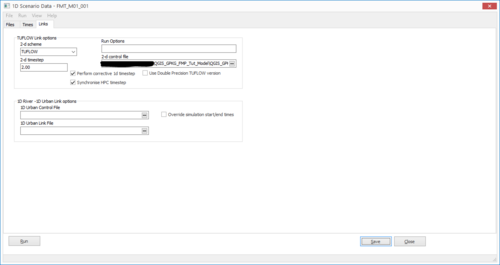
- Save the Scenario Data and run the Flood Modeller simulation.


Review Check Files
Review Boundaries and 1D/2D Links
From the TUFLOW\check\2d\ folder open within QGIS:
- FMT_M02_001_1d_to_2d_check
- FMT_M02_001_sac_check
The _1d_to_2d_check layer highlights the location of all 1D/2D boundary links within the model. In this case it should show the HX boundaries that have been digitised along the river banks.
The _sac_check layer highlights the lowest 2d cells within the SA boundary polygon to which inflow is first distributed.
Review Bank Elevations
From the TUFLOW\check\2d\ folder open within QGIS:
- FMT_M01_001_zln_zpt_check_P
The _zln_zpt_check layer highlights the cells whose elevations have been modified by z lines to represent the bank crests of the watercourse.
Review the Results
Instructions for viewing the TUFLOW mesh (XMDF) and 1D time series (.tpc) outputs are provided in Module 1 and Module 3. It is often useful to view 1D Flood Modeller results alongside 2D TUFLOW map outputs. The Flood Modeller results can be opened in QGIS with the TUFLOW Viewer plugin, together with the TUFLOW mesh results, by following the linked instructions. Alternatively, the TUFLOW mesh results can be loaded directly into the Flood Modeller Pro interface.
The video below demonstrates both methods:
- Loading Flood Modeller 1D results in QGIS using the TUFLOW Viewer plugin.
- Loading TUFLOW mesh results in Flood Modeller Pro.
Troubleshooting
Troubleshooting for HPC Simulation
If the following error message is encountered when running the TUFLOW HPC model:
ERROR 3999 - ptx file version mismatch
Please ensure that the four TUFLOW kernel files below have been transferred from your TUFLOW engine folder into your Flood Modeller "bin" folder.
- hpcKernels_nSP.ptx
- hpcKernels_nDP.ptx
- qpcKernels_nSP.ptx
- qpcKernels_nDP.ptx
Troubleshooting for GPU Simulation
If the following error is encountered when running the TUFLOW HPC model using GPU hardware: :
TUFLOW GPU: Interrogating CUDA enabled GPUs …
TUFLOW GPU: Error: Non-CUDA Success Code returned
or
ERROR 2785 - No GPU devices found, enabled or compatible.
Please try the following steps:
- Check if the GPU card is an NVIDIA GPU card. Currently, TUFLOW does not run on AMD type GPU.
- Check if the NVIDIA GPU card is CUDA enabled and whether the latest drivers are installed (see GPU Setup).
If an issue not described above is encountered, an email should be sent to support@tuflow.com.
| Up |
|---|