1D Pits

Introduction

There are predominantly two types of stormwater pits (drains/gullies) used as inlets to collect overland runoff and transfer that water to the underlying drainage/culvert/pipe network;

• Grated inlets
• Kerb Inlets (side entry pits / lintel inlets).

This page of the Wiki describes how pit inlet data is incorporated into a TUFLOW model.

Pit Inlet Types

Inlet Type	Example	Description
Q	Depth-Discharge Pit or Channel	Depth-Discharge Pit or Channel, pit inlet inflow information is defined within TUFLOW via a user defined Pit Inlet Database and associated pit inlet curves. This approach allows for unlimited flexibility. Any pit design or configuration can be incorporated into a TUFLOW model if the inlet depth-discharge relationship is known.
R	Kerb Inlet	Kerb inlets, also know as side entry pits or lintels are common in Australia. The pit chamber can vary depending on overall depth, length and the addition of any haunched riser units.
C	Circular Pit Inlet	Circular pit inlet
W	Grate (London, UK)	Grates, also known as Gully Pits, are common in the United Kingdom and are generally a square grate on top of a circular chamber and a riser outlet. The outlet will then feed into a larger culvert that forms part of the larger urban drainage network.

Pit Inlet Data Sources

Pit inlet depth-discharge data can be obtained from a variety of sources. The most common typically being from suppliers or local agencies who enforce consistent design standards within their jurisdiction. For demonstration purposes, examples from Sutherland Shire Council and Brisbane City Council are provided below.

Sutherland Shire Council

The Sutherland Shire Council Urban Drainage Manual (1992) includes summary tables and graphs documenting pit grate and lintel capacity information (derived from Department of Main Roads testing). The guidelines are compatible with the standard pit grate and lintel design shown below:

The capacity of a pit depends on three factors:

• The clear opening area of the grate
• The depth of water ponding over the grate
• The length of kerb inlet (lintel) opening

The following graphs summarise grate and lintel discharge estimates for a range of water depths and blockage factors, derived from the Sutherland Shire Council design standards.

The above graphs estimate unit length and area flow estimates. These unit values can be multiplied by real pit dimensions to define at site depth-discharge characteristics.

TUFLOW modelling requires the derivation of a unique depth-discharge curve for each pit type within the modelled area. An example is provided below for a single pit location.

Brisbane City Council

The pit inlet curve examples below originate from Brisbane City Council 8000 series standard drawings: https://www.brisbane.qld.gov.au/planning-building/planning-guidelines-tools/planning-guidelines/standard-drawings

South Australian Road Stormwater Drainage Inlets: Hydraulic Study (University of South Australia)

The Urban Water Resources Centre (UWRC) at the University of South Australia conducted a comprehensive set of hydraulic studies, examining performance of the most common roads’ stormwater drainage inlets in use in South Australia. The study was carried out using the Centre's unique full-scale road surface drainage test rig. Links to the pipe inlets curves are provided in the following link and sections below: Hydraulic Study (University of South Australia)

Transport South Australia

Transport South Australia Pit Inlet Curves

City of Adelaide

City of Adelaide Pit Inlet Curves

City of Campbelltown

City of Campbelltown Pit Inlet Curves

City of Charles Sturt

City of Charles Sturt Pit Inlet Curves

City of Onkaparinga

City of Onkaparinga Pit Inlet Curves

City of Playford

City of Playford Pit Inlet Curves

City of Port Adelaide / Enfield

City of Port Adelaide / Enfield Pit Inlet Curves

City of Marion

City of Marion Pit Inlet Curves

City of Mitcham

City of Mitcham Pit Inlet Curves

City of Salisbury

City of Salisbury Pit Inlet Curves

City of Tea Tree Gully

City of Tea Tree Gully Pit Inlet Curves

City of West Torrens

City of West Torrens Pit Inlet Curves

Spacing of Road Gullies (UK standards: BS EN 124 and BS7903)

The following section describes the Spacing of Road Gullies guidance (UK standards: BS EN 124 and BS 7903) which provides a method for determining road gulley capture rates.

The method depends on the following Hydraulic parameters:

• Longitudinal gradient, S_L, along the length of the scheme (expressed as fraction).

• Cross-fall, S_c (also expressed as a fraction).

• Manning’s roughness coefficient, n. Usually n = 0.017 for a conventional road surface. Other values are given in the following Table 1. (For more details, please see Section: 5, Table 5.3N of the guidance).

Table 1: Values of Manning's n

• The grating type (P, Q, R, S or T), or the size and angle of kerb inlet.

• The maximum allowable flow width (as shown below by B in m) against the kerb.

Calculation of Gully Flow Capture Rates based on Equations
The equations given in Appendix C (p.g: 25) of the guidance can be used to determine flow capture rates at different depths, to determine the depth-discharge curve for use within TUFLOW. The method requires the calculations of the flow capacity of the kerb channel and flow collection efficiency of the gully grate.

• As a first step, a gully grate type: P, Q, R, S or T should be selected. The selection of the grating type will determine the design value G_d (grating parameter) from Table 2. (For more details, please see Table A.2, Appendix A of the guidance).

Table 2: Determination of grating type G_d

• Road (longitudinal) gradient (S_L), Crossfall (S_c) and Manning's (n) should then be determined. Parameter values can be obtained from Table 3.

Table 3: Determination of S_L, S_c and Manning's n

• Further, a Water Depth against the kerb H (m) range should be provided. (Please note: The depth range can be changed, but the following equations that are used to calculate the flow capacity are only valid up to the kerb height).

• With the above parameters, the calculations of the i) Flow width (B in m), ii) Cross-sectional area (A_f in m2), iii) Hydraulic radius (R in m), iv) Flow rate (Q in m3/s) and v) Flow collection efficiency (ŋ (%)) based on the Equations C.1-C.5 which are presented in Appendix C of the guidance can be completed.

• Finally, the resulting depth-discharge data can be used in the TUFLOW pit inlet curves.
  

The Gully Flow Capture Rates template here, includes a calculation tab which can be used for the completion of the above calculation processes. Based on calculations and Equations C.6 and C.7 of the guidance the maximum allowable spacings upstream of the gully can be further calculated (For more details, please see Appendix C, p.g: 25).

Key assumption
Note: This method assumes that the route the flow takes around the trap limits the discharge from the gully pot to 10 l/s. This limit is effective in both directions, so any negative head on the gully would create -10 l/s flow back up through the gully and flood onto the road.

UK Water Industry Research (UKWIR) Inlet Capture Tool

In 2023, the UK Water Industry Research (UKWIR) Limited released the Modelling Sewer Inlet Capacity Restrictions Report Modelling Sewer Inlet Capacity Restrictions Report. The main aim was to develop a sewer modelling methodology to enable the representation of inlet inflow restrictions, focusing on the development of a new 1D model approach to provide more accurate model sewer flooding predictions. The new modelling approach has been devised by combining the findings from a literature review and the development of semi-empirical relationships from academic studies which investigated factors affecting inlet capacity. The new approach allows for 2 types of gully response reflecting 2 flow conditions: Subcritical flow on a shallow road gradient and Supercritical flow on a steep road gradients. A threshold of 0.02 is used to distinguish between shallow and steep road gradients. The reported equations can be used for the production of input inlet curves for TUFLOW 1D pit inlet modelling.

A template for the generation of the UKWIR Inlet Curve can be downloaded from here. The template determines both Subcritical Head-Discharge and Supercritical Head-Discharge relationships obtained from the Modelling Sewer Inlet Capacity Restrictions Report based on user input values of water depth (in metres). Two sets of curves can be generated, curves based on default parameters, and those based on user-defined parameters.

How to Translate On-Grade Approach Flow / Pit Capture Flow Curves to Depth / Discharge Curves for use in TUFLOW

Manning's equation calculations can be used to convert on-grade approach flow information to a water depth at the pit. ARR 2019 Guidelines (Section 5.6.1, Chapter 5, Book 9) recommends the use of the modified Mannings equation, the Izzard's equation, for gutter and roadway flow.

After manually calculating the depth to flow relationship the user simply needs to associate these water depth values with the pit capture flow information typically included in on grade pit inlet curve datasets.

TUFLOW Model Inputs

The steps required to represent pit inlet information within a TUFLOW model is summarised below:

1. Import an empty 1d_nwk GIS file from the TUFLOW file template folder (model\gis\empty).
2. Digitise points to represent pit locations. The points should be snapped to the start or end of 1d_nwk line features that define the underground pipe network.
3. Update the field attributes for each Pit point. Refer to 5.12.2 of the 2016 TUFLOW Manual. The most commonly used attributes are:
   • Type = Q (C, R and W are also options if pit inlets based on structure dimension is required instead of using a Pit Inlet Database approach).
   • US_Invert = Used to specify the ground elevation of the pit. If Conn_1D_2D is set to “SXL”, US_Invert is used as the amount by which to lower the 2D cell and the pit channel invert is set to this level.
   • DS_Invert = The bottom elevation of the pit. This input can also be used to set the upstream and downstream inverts of connected pipes/channels.
   • Inlet_Type = For Q pit channels, the name of a pit inlet type in the Pit Inlet Database. Multiple Pits can use the same Inlet_Type ID if they have the same design dimensions.
   • Conn_1D_2D = SXL can be specified to connect the 1D pit or node to the 2D domain and lower the 2D cell by the amount of the US_Invert attribute. The invert of the pit channel is set to the lowered 2D cell level. This is useful to help trap the water into the pit as it flows overland in the 2D domain. This feature works well in combination with the new Read GIS SA PITS option.
4. Update the Estry Control File (*.ecf) to include reference to the new 1d_nwk GIS file.
   Read GIS Network ==..\model\mi\Estry\1d_nwk_****.MIF
   
5. Create a Pit Inlet Database csv file. This file lists each type of pit (matching the names listed in the 1d_nwk "Inlet_Type" field). It also provides reference to the depth-discharge curve information.
   
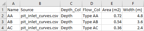
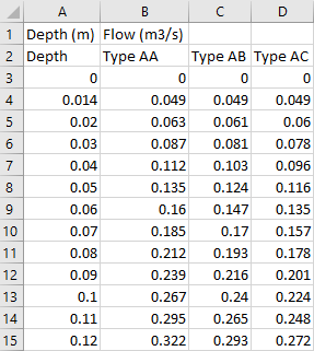
6. Create the Source file referenced in the Pit Inlet Database. The source file defines the depth-discharge information for each pit (determined from the relevant design standards). The column headers must match the entries in the Pit Inlet Database.
   
7. Update the Estry Control File (*.ecf) to include reference to the Pit Inlet Database.
   Pit Inlet Database ==..\pit_dbase\EG_pit_dbase.csv
   

An example model including Pits is available for download: https://wiki.tuflow.com/index.php?title=TUFLOW_Example_Models

Pit Search Distance

Some agency pit datasets may not have all pit point features snapped to the associated pipe line features. The *.ecf command "Pit Search Distance" can be useful in this instance. It automatically connects floating nodes to the 1D pipe network where connectors are not snapped to channel ends:

Pit Search Distance ==xxx
Read GIS Network ==..\model\mi\1d_nwke_*****.MIF

The order of the "Pit Search Distance" command is important as it can be repeated multiple times with different values that are assigned to the 1d_nwke(s) below the Pit Search Distance command. The pit search command should be included above the the GIS layer containing the pits.

To check if the Pit Search Distance is working as expected, import the *_nwk_C_check file to visually see if the pits are automatically connecting to a culvert. The image below is an example of the *_nwk_C_check file and the connections TUFLOW has made to each pit.

Any further questions please email TUFLOW support: support@tuflow.com

Up
Back to 1D Channels and Hydraulic Structures