Tutorial Module14 Archive: Difference between revisions
| Line 115: | Line 115: | ||
<li> Run the model. <br> |
<li> Run the model. <br> |
||
</ol> |
</ol> |
||
''TIP: To switch on the HPC solver via scenario control commands, please see the <u>[[ |
''TIP: To switch on the HPC solver via scenario control commands, please see the <u>[[Tutorial_Module05_Archive | HPC Model Setup]]</u> section of Module 5 (recommended).''<br> |
||
:''Also, to learn how to optimise a HPC simulation to achieve the fastest simulation speed please complete <u>[[ |
:''Also, to learn how to optimise a HPC simulation to achieve the fastest simulation speed please complete <u>[[Tutorial_Module02_Archive | Tutorial Module 2 ]]</u> and <u>[[Tutorial_Module03_Archive | Tutorial Module 3 ]]</u><br>'' |
||
==Results== |
==Results== |
||
Revision as of 15:41, 14 June 2022
- Start by copying the template boundary condition database, TUFLOW Tutorial Model BC Database.xls, from the Module_Data\Module_14\Excel folder into the TUFLOW\model\bc_dbase folder (keep the same file name). Open the file using Excel.
- With the 'bc_dbase' worksheet selected, enter the boundary name pump into cell A4. The name must appear exactly as it does in the 2d_bc_M14_pump layer so that TUFLOW knows where this boundary condition is to be applied in the model.
- The 'Source' column refers to the text file where the boundary data will be extracted from (to be created shortly). 'Column 1' and 'Column 2' specifies the columns in this text file where head and flow boundary data will be read from. Enter M14_pump_rates.csv in cell B4, head in cell C4 and flow in cell D4 as shown below.
- In Excel, switch to the 'M14_pump_rates' worksheet and review the flow versus head boundary that has been provided. Note that the boundary condition specifies pumping to commence when the water level at the 2D cell the pump is located at reaches 40.0 metres. The pumping rate rises to 0.25m3/s at 40.1 metres and continues steady at this rate for water levels above 40.1 metres. 50.0 metres has been specified as the upper limit and is above the highest water level expected for the simulation.
- If you haven't already, open the TUFLOW_tools_v2.0.xlam.
The process for adding these utilities to Excel, so that they open with Excel is detailed here: Excel Tips. To use these utilities without adding them to Excel simply open the TUFLOW_Tools_v2.0.xlam available in the Module_Data\Module_01\Excel folder.
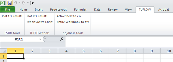
This should add a new menu in Excel titled TUFLOW. Navigate to this menu and select Entire Worksheet to csv to export all the M14 bc_dbase worksheets as .csv files to the TUFLOW\model\bc_dbase folder. - Save a copy of the boundary control file used in Module 3 (TUFLOW\model\M02_5m_001.tbc) as M14_5m_001.tbc in the TUFLOW\model\ folder.
- Open M14_5m_001.tbc in your text editor and add the following lines:
For MapInfo users add:
Read GIS BC == mi\2d_bc_M14_pump_001.MIF
For ArcGIS or QGIS users add:
Read GIS BC == gis\2d_bc_M14_pump_001_L.shp | gis\2d_bc_M14_pump_001_P.shp
- Using your text editor open and save a copy of the TUFLOW control file used in Module 3 (TUFLOW\runs\M03_5m_001.tcf) as M14_5m_001.tcf in the same folder.
- Note: There were no changes to the geometry for Module 14 and so the 2D geometry created in Module 3 is used.
- Change the reference to the Boundary Control File as follows:
BC Control File == ..\model\M14_5m_001.tbc
- Change the reference to the boundary database as follows:
BC Database == ..\bc_dbase\bc_dbase_M14.csv
- Change the Output Folder for Module 14 as follows: Output Folder == ..\results\M14\2d
- Using your preferred method, detailed in Module 1 Running TUFLOW, start TUFLOW. I am using a batch file to start TUFLOW and I simply double-click on this file in Windows Explorer. The simulation will take a few minutes to process (depending on the speed of you computer). This is a good time to complete your Modelling Log and keep a record of your work and TUFLOW simulations. Modelling logs are discussed here. A template modelling log is included in the TUFLOW Folders Template\TUFLOW\ folder supplied with this tutorial.
- Import/open the M14_5m_001_bcc_check layer located in the TUFLOW\check\2d\ folder. Confirm that you're happy with the 2D cell your pump is linked to and that the SH boundary cell attributes are as you intended.
- Using your text editor, open the Simulation Log (.tlf) and Simulation Summary (.tsf) files located in the TUFLOW\runs\log\ folder.
- These log files allow you to review all aspects of the model, in particular the cumulative mass error, number of negative depths that occurred and warnings that may have occurred prior to or during the simulation.
- Open the M14_5m_001_messages.csv file or import/open the M14_5m_001_messages GIS layer to your chosen GIS package. There should be no messages present, though this can vary slightly depending on the specific build of TUFLOW you are using.
- CHECK 2098 - Could not find a SC connection snapped to SH boundary.
- Why does the TUFLOW DOS Window open, though the TCF isn’t read and the simulation doesn’t execute?
- Save the TUFLOW runfile (M14_5m_001.tcf) as M14_5m_002.tcf.
- Add the following command and save the file:
- Solution Scheme == HPC ! Use HPC solver to run the model
- Solution Scheme == HPC ! Use HPC solver to run the model
- If you have a CUDA enabled NVIDIA GPU device, you can also add the following command to run the HPC solver using GPU hardware:
- Hardware == GPU ! Run HPC solver on GPU
- Hardware == GPU ! Run HPC solver on GPU
- Run the model.
- Also, to learn how to optimise a HPC simulation to achieve the fastest simulation speed please complete Tutorial Module 2 and Tutorial Module 3
- Check the simulation logs in the DOS window, .tlf and .hpc.tlf log files.
- View the results in your preferred package.
- Check if your GPU card is an NVIDIA GPU card. Currently, TUFLOW does not run on AMD type GPU.
- Check if your NVIDIA GPU card is CUDA enabled and whether the latest drivers are installed. Please see GPU Setup.
Introduction
This module focuses on adding a pump to the tutorial model to simulate pumping of water from one location in the model to another. The addition of pumps to a TUFLOW model is quick and easy, requiring the creation of a single additional GIS layer, a text file specifying the pumping rate and revision of a command in your model files.
This module builds upon Module 3. Module 3 is available from the Downloads section of the TUFLOW website. References will be made to various TUFLOW utilities that are similarly available from the TUFLOW website.
A pump constitutes an internal boundary condition to the model creating a transfer of flow, at a rate specified by the user, from one location in the 2D domain to another. The pump requires that a boundary condition be specified (2d_bc) of the flow versus head (SH) type. It is recommended that the user reads the relevant parts of section 4.10.7 of the 2010 TUFLOW manual (also available from the TUFLOW website).
Define New Boundary Conditions
At this stage we need to specify where the pump is located in the 2D domain and where the pumped flow is to be transferred to. The pump may be added as an additional boundary to a pre-existing 2d_bc boundary layer. For this tutorial a separate 2d_bc layer will be created for the pump.
Whilst grouping 2D boundaries into fewer 2d_bc layers will limit the number of GIS layers in your model, locating groups of boundary types into separate files will enable you to easily turn on and off particular boundaries in different simulations of your model without having to revert to editing your GIS layers.
For details on setting up the required GIS layer, please select your GIS package.
Modify Simulation Control Files and Boundary Condition Database
With the new GIS layer created it is time to update the control files and boundary condition database (bc_dbase). The files we need to change are the bc_dbase (.csv), TUFLOW boundary condition file (.tbc) and the TUFLOW control file (.tcf).
Boundary Condition Database
The bc_dbase contains an entry for each boundary condition and a new entry is required for the pump. The boundary condition for the pump will link to a text file (.csv) that specifies the pump rate (flow) controlled by the water level (head).


TBC File
The newly created 2d_bc_M14_pump_001 layer(s) need to be added to the TUFLOW boundary control file (.tbc).
TCF File
A new TUFLOW control file (.tcf) is required for Module 14 that includes reference to the new .tbc file and an updated filepath for saving model results.
You do not need to add the comments that follow exclamation marks. These commands are generally self explanatory. However for this tutorial model they are included.
Save your .tcf file. You're now (hopefully!) ready to try simulating the Module 14 TUFLOW model.
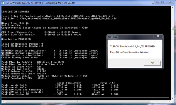
If your simulation has been successful, the console window should look similar to the image below.

Reviewing Check Files and Model Performance
Check Files
The 2D boundary condition check file shows the 2D model cell that the pump is linked to and from where flow is removed.
Model Performance
As we did with Module 1, it is highly recommended that you review the model's performance. Hydraulic models are able to do unexpected things even if the simulation completes successfully!
Reviewing Results
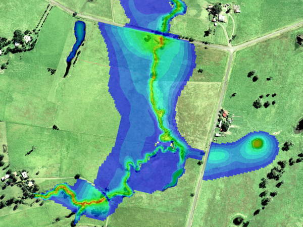
The TUFLOW model 2D results may be viewed in a number of software packages. Follow the method for your software package(s) described in Module 1 Viewing the Results to analyse the results and view the pump operation.
The image below has been taken from SMS and shows the pumped flow taken from the creek has been transferred to the dam to the west.

Conclusion
We have used the SH 2D boundary type to add a pump to the TUFLOW model. The addition of a pump to a TUFLOW model is easily done and allows the simulation of pumping from one location to another at a rate specified by the user, with the pump flow controlled by the water level at the location of the pump.
Troubleshooting
This section contains a link to some common problems that may occur when progressing through Module 14 of the TUFLOW tutorial model.
If you experience an issue that is not detailed, please email support@tuflow.com or add and describe the problem on the discussion page.
Advanced - HPC Solver (Optional)
This section will introduce how to run the model TUFLOW’s HPC (Heavily Parallelised Compute) solver, and how to fix some common issues that may occur when trying to run a simulation using Graphics Processing Unit (GPU) hardware.
TUFLOW HPC can run between 10 and 100 times faster than TUFLOW Classic using NVidia Graphics Processing Units (GPU)(depending on the model configuration and hardware performance).
Model Setup
In order to use the HPC solver, we will need to perform the following steps:
TIP: To switch on the HPC solver via scenario control commands, please see the HPC Model Setup section of Module 5 (recommended).
Results
Using the methods described above in the Viewing Results section of Module 1.
Do the logs and results appear different to the TUFLOW Classic simulation?
Troubleshooting for GPU Simulations
If you receive the following error when trying to run the TUFLOW HPC model using GPU hardware:
TUFLOW GPU: Interrogating CUDA enabled GPUs …
TUFLOW GPU: Error: Non-CUDA Success Code returned
or
ERROR 2785 - No GPU devices found, enabled or compatible.
Please try the following steps:
If you experience an issue that is not detailed above please send an email to support@tuflow.com