Tutorial M06
Introduction
In this module, a direct rainfall model is built. The tutorial demonstrates three ways of modelling rainfall for a direct rainfall approach.
- Part 1: Global Rainfall - apply uniform rainfall to all active cells.
- Part 2: Rainfall Polygons - apply rainfall to active cells within digitised polygons and losses within the materials layer.
- Part 3: Gridded Rainfall - apply rainfall temporally and spatially using a TUFLOW Rainfall Control File (TRFC).
The GIS layers are:
- TBC layers:
- 2d_rf: polygons are assigned a rainfall gauge and spatial and temporal adjustment factors.
- TRFC layers:
- 2d_rf: points are specified reflecting rainfall gauge locations. Rainfall is interpolated and a series of rainfall grids are generated.
Module 6 builds from the model created in Module 2. The completed Module 2 model is provided in the Module_06\TUFLOW folder.
Part 1 - Global Rainfall
Boundary Condition Database (bc_dbase)
Update the bc_dbase with a reference to the new rainfall hyetographs:
- Navigate to the Module_06\Tutorial_Data folder. Copy the rainfall_stations.csv and paste it in the Module_06\TUFLOW\bc_dbase folder. This file contains the rainfall hyetographs.
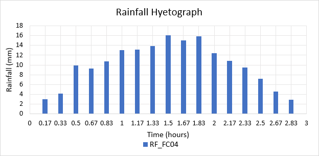
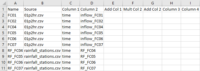
- Open the file, there are 4 columns labelled ‘RF_FC04’ to ‘RF_FC07’. Part 1 references 'RF_FC04', the remaining hyetographs are used in Part 2.
- Save a copy of the bc_dbase.csv as bc_dbase_M06_001.csv.
- Open the file and add the additional rainfall boundary conditions as shown below:
- Save the bc_dbase.


Materials
Surface roughness or bed resistance values (e.g. Manning’s n) are assigned to material IDs. Depth varying roughness values are used in direct rainfall models to reflect the bed roughness at shallow depths.
- Copy the materials_M06_001.csv file from the Module_06\Tutorial_Data folder into the Module_06\TUFLOW\model folder. Depth varying roughness values are applied to three of the Material IDs within the study area:
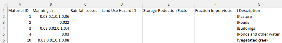
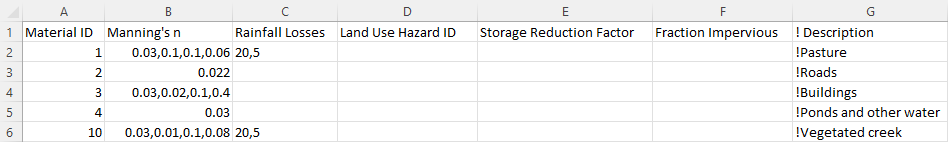
- For Material ID 1, 3 and 10, four numbers (y1, n1, y2, n2) are added to each row separated by commas and are applied as follows:
- Below depth y1 (m), a Manning’s n value of n1 is applied.
- Above depth y2 (m), a Manning’s n value n2 is applied.
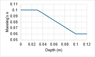
- Between y1 and y2, the Manning’s n value is interpolated between n1 and n2. The default interpolation method uses a curved fit so that the n values transition gradually.
- For example, for Material ID 1, for depths of water below 0.03m a Manning's n value of 0.10 is applied. For depths of water greater than 0.1m, a Manning's n value of 0.06 is applied. Between 0.03 to 0.1m, a Manning's n value is interpolated between 0.1 and 0.06:
- For Material ID 2 and 4, the Manning’s n value specified in the second column will be applied at all depths, i.e. a value of 0.022 for Material ID 2.


Simulation Control Files
TUFLOW Boundary Control File (TBC)
- Save a copy of M01_001.tbc as M06_001.tbc in the Module_06\TUFLOW\model folder.
- Open the M06_001.tbc in a text editor.
- The current rainfall versus time inflows (2d_sa) are replaced in this tutorial. The base inflow and outflow (2d_bc) remain the same. Comment out the 'Read GIS SA' command by placing '!' at the beginning:
QGIS - SHP
! Read GIS SA == gis\2d_sa_M01_001_R.shp
QGIS - GPKG
! Read GIS SA == 2d_sa_M01_001_R
- Add the following command line:
Global Rainfall BC == RF_FC04 ! Reads in global rainfall - Save the TBC.
The Global Rainfall BC command applies a rainfall depth to every active cell within the 2d_code layer based on the input hyetograph. In this case it is the 'RF_FC04' hyetograph specified in the rainfall_stations.csv. The input hyetograph must be in mm verse time, and is applied using a stepped approach. The stepped approach holds the rainfall constant for the time interval (i.e. the rainfall has a histogram stair-step shape). This means, for example, the second rainfall value in the time-series is applied as a constant rainfall from the first time value to the second time value. As with all rainfall boundaries, the first and last rainfall entries should be set to zero, otherwise these rainfall values are applied as a constant rainfall if the simulation starts before or extends beyond the first and last time values in the rainfall time-series.
TUFLOW Control File (TCF)
- Save a copy of M02_5m_001.tcf as M06_5m_001.tcf in the Module_06\TUFLOW\runs folder.
- Open the M06_5m_001.tcf in a text editor and make the following reference updates:
BC Control File == ..\model\M06_001.tbc ! Reference the TUFLOW Boundary Conditions Control File
BC Database == ..\bc_dbase\bc_dbase_M06_001.csv ! Reference the Boundary Conditions Database
Read Materials File == ..\model\materials_M06_001.csv ! Reference the Materials Definition File
- A Timestep Maximum command is required in direct rainfall modelling to ensure the timestep does not get too large during periods where cells are dry (causing the model to become unstable). Include the command in the 'Time Control' section:
Timestep Maximum == 2.5 ! Specifies a maximum timestep of 2.5 seconds
- Add Cumulative Rainfall (RFC), Rainfall Rate (RFR) and Manning's n (n) as additional Map Output Data Types. These outputs are discussed in the Results section.
Map Output Data Types == h V d dt RFC RFR n ! Outputs water levels, velocities, depths, minimum timestep, cumulative rainfall, rainfall rate, manning's n
- A Map Cutoff Depth is useful for direct rainfall modelling where there is a need to differentiate between very shallow sheet flow and flooding. Include the following command in the ! OUTPUT SETTINGS section:
Map Cutoff Depth == 0.05 ! Sets map cutoff depth of 0.05 meters
- Save the TCF.
Running the Simulation
- Save a copy of _run_M02_HPC.bat as _run_M06_HPC.bat in the Module_06\TUFLOW\runs folder.
- Update the batch file to reference the M06_5m_001.tcf :
set exe="..\..\..\exe\2023-03-AF\TUFLOW_iSP_w64.exe"
set run=start "TUFLOW" /wait %exe% -b
%run% M06_5m_001.tcf
- Save the batch file and double click it in file explorer to run the simulation.
Troubleshooting
See tips on common mistakes and troubleshooting steps if the model doesn't run:
Check Files
While the model is running, review the added features are specified correctly:
- Open the M06_5m_001.tlf from the Module_06\TUFLOW\runs\log folder in a text editor.
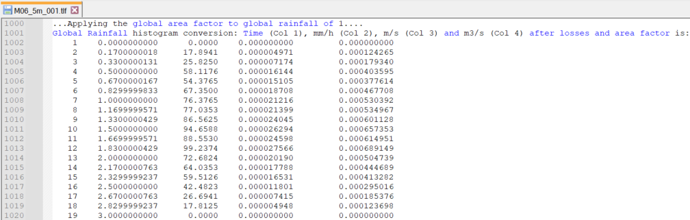
- Review the hyetograph information. When using the direct rainfall approach, a rainfall depth fallen in a particular increment of time is input. TUFLOW converts this depth per time increment to a flow (m3/s) and applies this flow at each cell. The TLF shows this conversion:

Results
When the model is finished, review the results:
Part 2 - Rainfall Polygons
The second part of this module introduces:
- Polygons in a 2d_rf file to distribute multiple hyetographs across the catchment.
- Initial and continuing rainfall losses in the materials file.
GIS Inputs
Create, import and view input data:
Materials
Rainfall losses applied through the materials file remove the loss depth from the rainfall before it is applied as a boundary on the 2D cells.
- Save a copy of materials_M06_001.csv as materials_M06_002.csv in the Module_06\TUFLOW\model folder.
- Open the materials_M06_002.csv in a spreadsheet program.
- Update the Rainfall Losses column for Material 1D 1 (pasture) and 10 (vegetated creek) with an initial loss of 20mm and continuing loss of 5mm/hr:
- Save the materials file.

Simulation Control Files
TUFLOW Boundary Control File (TBC)
- Save a copy of M06_001.tbc as M06_002.tbc in the Module_06\TUFLOW\model folder.
- Open the M06_002.tbc in a text editor.
- Comment out the Global Rainfall command and add the Read GIS RF command:
QGIS - SHP
! Global Rainfall BC == RF_FC04
Read GIS RF == gis\2d_rf_M06_polygons_002_R.shp ! Reads in 2D rainfall boundaries
QGIS - GPKG
! Global Rainfall BC == RF_FC04
Read GIS RF == 2d_rf_M06_polygons_002_R ! Reads in 2D rainfall boundaries
- Save the TBC.
TUFLOW Control File (TCF)
- Save a copy of M06_5m_001.tcf as M06_5m_002.tcf in the Module_06\TUFLOW\runs folder.
- Open the M06_5m_002.tcf in a text editor and make the following reference updates:
QGIS - SHP
BC Control File == ..\model\M06_002.tbc ! Reference the TUFLOW Boundary Conditions Control File
Read Materials File == ..\model\materials_M06_002.csv ! Reference the Materials Definition File
QGIS - GPKG
Spatial Database == ..\model\gis\M06_002.gpkg ! Specify the location of the GeoPackage Spatial Database
BC Control File == ..\model\M06_002.tbc ! Reference the TUFLOW Boundary Conditions Control File
Read Materials File == ..\model\materials_M06_002.csv ! Reference the Materials Definition File
- Add Material Rainfall Loss (RFML) as an additional Map Output Data Type. This output is discussed in the Results section.
Map Output Data Types == h V d dt RFC RFR n RFML ! Outputs water levels, velocities, depths, minimum timestep, cumulative rainfall, rainfall rate, material based rainfall loss - Save the TCF.
Running the Simulation
Update the batch file created in the first part of Module 6 to reference the M06_5m_002.tcf file. Save the batch file and double click it in file explorer to run the simulation.
Troubleshooting
See tips on common mistakes and troubleshooting steps if the model doesn't run:
Check Files
While the model is running, review the added features are specified correctly:
- Open the M06_5m_002.tlf from the Module_06\TUFLOW\runs\log folder in a text editor.
- Review the losses applied in the materials layer:
- Review the hyetograph information. The TLF shows the conversion for each histogram:
Results
When the model is finished, review the results:
Part 3 - Rainfall Control File
GIS Inputs
Create, import and view input data:
Simulation Control Files
TUFLOW Rainfall Control File (TRFC)
The TRFC commands generate rainfall grids based on point rainfall gauges. There are three spatial interpolation methods available, this tutorial uses Inverse Distance Weighting (IDW). For more information on IDW and the other available methods, refer to the TUFLOW Manual or TUFLOW Rainfall Control File Examples.
The TRFC is processed during model initialisation, outputting a series of rainfall grids which are used by the simulation to vary the rainfall over the 2D domain. The rainfall grids are output to a separate folder RFG\<TCF name> in the location of the TRFC (e.g. Module_06\TUFLOW\model\RFG\M06_5m_003). This approach reduces memory usage while TUFLOW is running.
- Create a new text file M06_point2grid_003.trfc and save it in the Module_06\TUFLOW\model folder.
- Add the following commands:
QGIS - SHP
RF Grid Format == TIF ! Sets the output grid format
RF Interpolation Method == IDW ! Sets the interpolation approach between rainfall locations
RF Grid Cell Size == 25 ! Sets the cell size for the generated rainfall grids
Read GIS RF Points == gis\2d_rf_M06_pt2grid_003_P.shp ! Reads the point rainfall locations in the 2d_rf file format
QGIS - GPKG
RF Grid Format == TIF ! Sets the output grid format
RF Interpolation Method == IDW ! Sets the interpolation approach between rainfall locations
RF Grid Cell Size == 25 ! Sets the cell size for the generated rainfall grids
Read GIS RF Points == 2d_rf_M06_pt2grid_003_P ! Reads the point rainfall locations in the 2d_rf file format
- Save the TRFC.
TUFLOW Boundary Control File (TBC)
- Save a copy of M06_002.tbc as M06_003.tbc in the Module_06\TUFLOW\model folder.
- Open the M06_003.tbc in a text editor and comment out the Read GIS RF command:
QGIS - SHP
! Read GIS RF == gis\2d_rf_M06_polygons_002_R.shp
QGIS - GPKG
! Read GIS RF == 2d_rf_M06_polygons_002_R
- Save the TBC.
TUFLOW Control File (TCF)
- Save a copy of M06_5m_002.tcf as M06_5m_003.tcf in the Module_06\TUFLOW\runs folder.
- Open the M06_5m_003.tcf in a text editor and make the following reference updates:
QGIS - SHP
BC Control File == ..\model\M06_003.tbc ! Reference the TUFLOW Boundary Conditions Control File
QGIS - GPKG
Spatial Database == ..\model\gis\M06_003.gpkg ! Specify the location of the GeoPackage Spatial Database
BC Control File == ..\model\M06_003.tbc ! Reference the TUFLOW Boundary Conditions Control File
- Include a reference to the TRFC in the Model Inputs section:
Rainfall Control File == ..\model\M06_point2grid_003.trfc ! Reference the TUFLOW Rainfall Control File
- Save the TCF.
Running the Simulation
Update the batch file to reference the M06_5m_003.tcf file. Save the batch file and double click it in file explorer to run the simulation.
Troubleshooting
See tips on common mistakes and troubleshooting steps if the model doesn't run:
Check Files
While the model is running, review the added features are specified correctly:
- Navigate to the Module_06\TUFLOW\model\RFG\M05_5m_003 folder with rainfall grids created from the rainfall interpolation.
- The timestep matches the one specified in the rainfall hyetographs (10 minutes). Hours are used in the rainfall grids names:

- A total rainfall depth M06_5m_003_rf_total.tif is created, this is not used by TUFLOW during the simulation, but can be used for checking purposes.

Results
When the model is finished, review the results:
Conclusion
- Direct rainfall approach was used in three ways - applied globally, to separate polygons using 2d_rf layer and varying temporally and spatially using a TUFLOW Rainfall Control (TRFC).
- Depth varying material values were used.
- Rainfall losses were applied in the materials layer.
- TUFLOW log files and rainfall grids were used to check the rainfall was applied correctly.
- Map outputs RFC, RFR, n and RFML were inspected.
Gridded Rainfall (Optional)
The rainfall grids created from the rainfall interpolation and located in the Module_06\TUFLOW\model\RFG\M06_5m_003 folder can be used by the Read Grid RF command in the TCF to apply the rainfall to the model, rather than regenerate the rainfall grids using the TRFC file (as long as the input files remain unchanged). The command references a csv file containing links to the rainfall grids.
- Navigate to the Module_06\Tutorial_Data folder. Copy the M06_004_rf.csv into the Module_06\TUFLOW\bc_dbase folder.
- Open the csv. The file requires two columns, the first is time (in simulation hours) and the second is the rainfall grid.
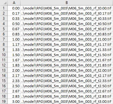
- Save a copy of M06_5m_003.tcf as M06_5m_004.tcf. Change the commands to read in the grids created in the RFG folder:
! Rainfall Control File == ..\model\M06_point2grid_003.trfc ! Reference the Rainfall Control File
Read Grid RF == ..\bc_dbase\M06_004_rf.csv
- Save the TCF, update the batch file and run the model.
- Compare the results with the Part 3 results.
- Check the run times in the _ TUFLOW Simulations.log from the TUFLOW\runs folder. For large models, the initialisation time is faster with the gridded rainfall set up.

| Up |
|---|