TUFLOW CATCH Tutorial M01
Introduction
In this module, a TUFLOW CATCH pollutant export model is developed.
TUFLOW CATCH Tutorial 01 is built from the model created in TUFLOW Tutorial Module 6 - Part 3. The completed TUFLOW Module 6 (part 3) is provided in the TUFLOW_CATCH_Module_01\Modelling\TUFLOW folder of the download dataset as the starting point for this tutorial. If unfamiliar with TUFLOW, it is recommended to complete Modules 1, 2, 3 and 6 of the TUFLOW Tutorials to establish an understanding of 1D and 2D TUFLOW modelling, including direct rainfall models.
Project Initialisation
TUFLOW CATCH models are separated into a series of folders which contain the input and output files. The recommended directory structure for TUFLOW CATCH models consists of a top-level folder, Modelling, which contains three subfolders:
- TUFLOW: Contains TUFLOW HPC input files.
- TUFLOWCATCH: Contains the TUFLOW CATCH Control file, as well as all check, results and log files.
- TUFLOWFV: Contains TUFLOW FV input files.
The third level subfolders are outlined below. For a more detailed description, refer to the TUFLOW CATCH Manual. For more information on TUFLOW HPC or TUFLOW FV folder structures, refer to the TUFLOW Manual or the TUFLOW FV Manual.

| Folder | Sub-Folder (s) | Description |
|---|---|---|
| TUFLOW | bc_dbase model |
Follows standard TUFLOW structure. |
| catch | Not used, but generated for internal use. It holds files that are produced during computation, but deleted when the simulation finishes successfully. | |
| check results runs |
Not used, but generated for internal use. All TUFLOW check and results files are written to the TUFLOWCATCH\check folder and the TUFLOWCATCH\results folder respectively. TUFLOW CATCH simulations are run from the .tcc file in the TUFLOWCATCH\runs folder. | |
| TUFLOWCATCH | bc_dbase | Contains the output boundary condition and time-series data. |
| check | Contains the GIS and other check files produced by TUFLOW CATCH, TUFLOW and TUFLOW FV to carry out quality control checks | |
| model | Not used - generated for internal use. | |
| results | Contains the result files produced by TUFLOW CATCH, TUFLOW and TUFLOW FV. | |
| runs | Contains the .tcc simulation control file. | |
| runs\log | Contains the log files (e.g. .catchlog, .tlf, .log, etc) and _messages.shp files produced by TUFLOW CATCH, TUFLOW and TUFLOW FV. | |
| TUFLOWFV | bc_dbase model stm wqm |
Follows standard TUFLOW FV structure. |
| check results runs |
Not used, but generated for internal use. All TUFLOW FV check and results files are written to the TUFLOWCATCH\check folder and the TUFLOWCATCH\results folder respectively. TUFLOW CATCH simulations are run from the .tcc file in the TUFLOWCATCH\runs folder. |
The TUFLOW CATCH folders can be set up manually, or automatically through the TUFLOW QGIS Plugin (recommended).
GIS Inputs
Create, import and view input data:
TUFLOW Boundary Condition Database (bc_dbase)
Update the bc_dbase to remove the 2D boundaries and add a reference to the timeseries temperature data. Note that TUFLOW CATCH does not support 2D boundaries, however, 2d_sa GIS layers can be used to simulate non-hydrologic surface loads. For more information on 2d_sa inputs, refer to Section 3.4 of the TUFLOW CATCH Manual.
- In Windows File Explorer, navigate to the TUFLOW_CATCH_Module_01\Tutorial_Data folder. Copy the temperature.csv and paste it in the TUFLOW_CATCH_Module_01\Modelling\TUFLOW\bc_dbase folder. This file contains the timeseries temperature data.
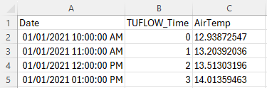
- Open the file. As this file will be read by TUFLOW CATCH, the first column must contain the date in ISODATE format (DD/MM/YYYY hh:mm:ss). It will also be read by TUFLOW HPC, and therefore must have a column specifying a time in hours from the beginning of the model. In this case, the 'TUFLOW_Time' column contains the time in hours. For example, 01/01/2021 10:00:00 corresponds to 0, 01/01/2021 11:00:00 to 1, and so on.
- In the TUFLOW\bc_dbase folder, save a copy of the bc_dbase_M06_001.csv as bc_dbase_TC01_001.csv.
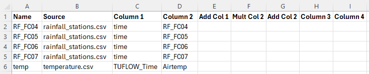
- Open the file and remove the references to the 2D boundaries (FC01, FC02, FC04, FC05, FC06 and FC07).
- Add the reference to the timeseries temperature data as shown below:
- Save the bc_dbase.


Materials
Surface roughness or bed resistance values (e.g. Manning’s n) are assigned to material IDs. To simulate a more complex catchment area, more material IDs have been specified.
- In Windows File Explorer, navigate to the TUFLOW_CATCH_Module_01\Tutorial_Data folder. Copy the materials_TC01_001.csv and paste it in the TUFLOW_CATCH_Module_01\Modelling\TUFLOW\model folder. This file is a modified version of materials_M06_002.csv from TUFLOW Tutorial Module 6.
- Open the file. Roughness values (Manning's n) have been applied to the five new material IDs:
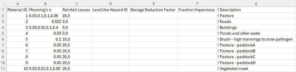
- These new material IDs have been assigned to allow different pollutant export properties to be specified to each material ID. This is discussed in the TUFLOW CATCH Control File section.

TUFLOW Soil File (.tsoilf)
The soils (.tsoilf) file is similar to the materials file. A positive integer ID is assigned to each soil, then an infiltration method followed by the soil parameters. For this tutorial, there is only one soil type (ID 1) which is applied across the whole model.
- In Windows File Explorer, navigate to the TUFLOW_CATCH_Module_01\Tutorial_Data folder. Copy the TC01_soils_001.tsoilf and paste it in the TUFLOW_CATCH_Module_01\Modelling\TUFLOW\model folder.
- Open the file. The Green-Ampt (GA) infiltration method has been used. For more information on infiltration methods, refer to the TUFLOW Manual.

Simulation Control Files
The following steps will require use of a text editor. The tutorial demonstration uses Notepad++. For its configuration information refer to Notepad++ Tips.
TUFLOW Geometry Control File (TGC)
- Save a copy of M02_001.tgc as TC01_001.tgc in the TUFLOW_CATCH_Module_01\Modelling\TUFLOW\model folder.
- Open the TC01_001.tgc in a text editor and add the following line after the 'Read GIS Mat' command to reference the new materials GIS layer.
Read GIS Mat == gis\2d_mat_TC01_001_R.shp ! Sets material values according to attributes in the GIS layer
- Add the following section to globally set the soil ID and the soil thickness:
! SOILS
Set Soil == 1 ! Globally sets the soil ID to 1
Set Soil Thickness == 0.2 ! Globally sets the soil thickness to 0.2m
- Save the TGC.
TUFLOW Boundary Control File (TBC)
- Save a copy of M06_003.tbc as TC01_001.tbc in the TUFLOW_CATCH_Module_01\Modelling\TUFLOW\model folder.
- Open the TC01_001.tbc in a text editor and remove or comment out the reference to the 2D boundaries using a '!' symbol.
! Read GIS BC == gis\2d_bc_M01_001_L.shp ! Reads in downstream 2D boundary
- Add the additional lines to reference the 1D/2D culvert connections:
Read GIS BC == gis\2d_bc_M03_culverts_001_P.shp ! Links the 1D culverts to the 2D domain
Read GIS BC == gis\2d_bc_M03_culverts_001_R.shp | gis\2d_bc_M03_culverts_001_L.shp ! Links the 1D culverts to the 2D domain
- Save the TBC.
TUFLOW ESTRY Control File (ECF)
- Navigate to the TUFLOW_CATCH_Module_01\Modelling\TUFLOW\model folder, and open TC01_001.ecf in a text editor. This file was created using the TUFLOW CATCH plugin.
- In the '1D Time Control' section, ensure the following command has been specified to set the 1D computational timestep:
Timestep == 0.5 ! Specifies a 1D computational timestep of 0.5 seconds
- In the '1D Elements' section, add the following command to define the culverts:
Read GIS Network == gis\1d_nwk_M03_culverts_001_L.shp ! Defines culverts - Add the following command line to define the Advection Dispersion (AD) approach. For more information on Advection Dispersion, please refer to the TUFLOW Manual.
AD Approach == METHOD A ! Sets the modelling approach for the Advection Dispersion through 1D channels - Save the ECF.
TUFLOW CATCH Control File (TCC)
A TUFLOW CATCH simulation is set up and executed by constructing a TUFLOW CATCH Control file (.tcc). TUFLOW Control file (.tcf) and TUFLOW FV Control file (.fvc) are not used. The .tcc has four command blocks:
- Global settings
- Catchment Hydraulic Model (TUFLOW HPC) commands
- Catchment Pollutant Export Model
- Receiving Model (TUFLOW FV) commands
All blocks must be included in the above order, but the later three can be switched on and off with a single command.
The TUFLOW CATCH plugin has created a .tcc template file in the TUFLOWCATCH\runs folder, TC01_001.tcc. This file has been populated with all the commands needed to execute a TUFLOW CATCH simulation. In this section, the template commands will be populated/updated for this tutorial model.
Global Settings
This section contains information that is applied equally to both TUFLOW HPC and TUFLOW FV.
- Navigate to the TUFLOW_CATCH_Module_01\Modelling\TUFLOWCATCH\runs folder and open TC01_001.tcc into a text editor.
- In the 'Simulation Settings' section, update the time commands:
Start Time == 01/01/2021 10:00:00 ! Specifies the simulation start time
End Time == 01/01/2021 13:00:00 ! Specifies the simulation end time
- In the 'Boundary Condition Configuration' section, update the BC and CSV output intervals:
Catch BC Output Interval Nodestring == 300 ! Outputs BC nodestring data every 300 seconds
Catch BC Output Interval Lateral == 300 ! Outputs BC lateral data every 300 seconds
CSV Write Frequency Day == 0.01 ! Writes CSV output every 0.01 days
Catchment Hydraulic Model (TUFLOW HPC)
This block contains commands that construct the TUFLOW HPC simulation. These commands are almost entirely those that would be used in setting up a standalone TUFLOW HPC control file (.tcf), with a small number of additional commands that relate to TUFLOW CATCH.
- Set the catchment hydraulic model:
Catchment Hydraulic Model == HPC - Set the zero date. TUFLOW HPC does not support ISODATE format, while TUFLOW FV requires it. This command ensures compatibility by setting the date in TUFLOW FV ISODATE format that corresponds to zero hours in TUFLOW HPC boundary condition files.
Zero Date == 01/01/2021 10:00 ! Specifies the simulation start time in TUFLOW FV ISODATE format
- In the 'GIS' section, remove or comment out the following command using a '!' symbol. The SHP projection has already been set in the Global Settings section.
! SHP Projection == ..\..\TUFLOW\model\gis\projection.shp
- In the 'GIS' section, set the projection for the output grid files:
TIF Projection == ..\..\TUFLOW\model\grid\DEM.tif ! Sets the GIS projection for the output grid files
- In the 'Solver' section, set the timestep maximum and time format:
Timestep Maximum == 2.5 ! Specifies a maximum timestep (seconds)
Time Format == TUFLOWFV ! Specifies the time format of output results
- In the 'SGS' section, set the sample target distance:
SGS Sample Target Distance == 0.5 ! Sets SGS Sample Target Distance (meters)
- In the 'Control Files' section, ensure all control files are referenced.
Geometry Control File == ..\..\TUFLOW\model\TC01_001.tgc ! Reference the TUFLOW Geometry Control File
BC Control File == ..\..\TUFLOW\model\TC01_001.tbc ! Reference the TUFLOW Boundary Conditions Control File
BC Database == ..\..\TUFLOW\bc_dbase\bc_dbase_TC01_001.csv ! Reference the Boundary Conditions Database
Read Materials File == ..\..\TUFLOW\model\materials_TC01_001.csv ! Reference the Materials Definition File
Rainfall Control File == ..\..\TUFLOW\model\M06_point2grid_003.trfc ! Reference the TUFLOW Rainfall Control File
ESTRY Control File == ..\..\TUFLOW\model\TC01_001.ecf ! Reference the ESTRY (1D) Control File
- In the 'Soils' section, reference the soils file (.tsoilf), and remove or comment out the 'soil negative rainfall approach' command using a '!' symbol.
Read Soils File == ..\..\TUFLOW\model\TC01_soils_001.tsoilf ! Reference the Soils File
! Soil Negative Rainfall Approach == FACTOR
- In the 'Pollutant Configuration' section, reference the receiving polygon and set the pollutants. In this tutorial, salinity, temperature, dissolved oxygen (WQ_DISS_OXYGEN_MG_L), alive and dead ecoli (WQ_PATH_ECOLI_ALIVE/DEAD_CFU_100ML) and clay sediment (SED_CLAY) are simulated.
Receiving Polygon == ..\..\TUFLOW\model\gis\2d_rp_TC01_001_R.shp ! GIS layer defining the receiving polygon
Pollutant == Salinity, Temperature, WQ_DISS_OXYGEN_MG_L, WQ_PATH_ECOLI_ALIVE_CFU_100ML, WQ_PATH_ECOLI_DEAD_CFU_100ML, SED_CLAY ! Specify the pollutant names
- In the 'Output Map Configuration' section, update the following commands to set the map output formats, the map output interval, map cuttoff depth and to define the TIF output parameters.
Map Output Format == XMDF TIF ! Result file types
Map Output Data Types == catch h v d ! Output data types
Map Output Interval == 30 ! Interval of output map data (seconds)
Map Cutoff Depth == 0.05 ! Sets map cutoff depth (meters)
TIF Map Output Interval == 0 ! Interval of output TIF map data (seconds)
TIF Map Output Data Types == h d dt ! TIF result file types
Pollutant Export Model
This block contains commands that control the pollutant export (and other constituent) simulation.
- Set the pollutant export model:
Catchment Pollutant Export Model == Mass Accumulation Release - In the 'Constant Concentrations' section, add the following commands. They set the pollutants 'Salinity' and 'WQ_DISS_OXYGEN_MG_L' (dissolved oxygen) to a constant concentration value that is applied equally to all boundaries and summary files where appropriate.
Constant Salinity == 0.0 ! Specify the constant concentration of salinity
Constant WQ_DISS_OXYGEN_MG_L == 8.0 ! Specify the constant concentration of dissolved oxygen
- In the 'Time Series' section, add the following command. It sets the pollutant 'Temperature' to be a time-series input, and points to the name 'temp' in the bc_dbase.
Time-Series Temperature == temp ! Specify temperature as a timeseries and the corresponding BC database name
- In the 'Pollutant Export Properties' section, add the material block 'ALL' (Material == ALL) from the page linked below. This code block defines the default pollutant export properties for each pollutant. Once uniform conditions are set, progressive specifications of material by material pollutant behaviour can be set. These specifications override previous settings on a spatial basis. Including the default (ALL) material block is considered best practice, as it ensures that all pollutants have export properties defined across the entire TUFLOW HPC domain, otherwise an error will occur. For more information on the pollutant export parameters, refer to Section 4.5.3.3 of the TUFLOW CATCH Manual.
- To set the pollutant export properties for the different material IDs, blocks similar to the above (e.g. Material == 4) can be used. The material IDs correspond to those defined in the 2d_mat_TC01_001.shp and 2d_mat_M01_001.shp GIS layers.
To estimate E. coli export rates for each paddock, the area of each paddock was calculated. Based on this, appropriate animal populations were assigned. Using these values, the E. coli rates were calculated. For more information on pollutant export calculations, refer to Section 3.2.3 of the TUFLOW CATCH Manual.
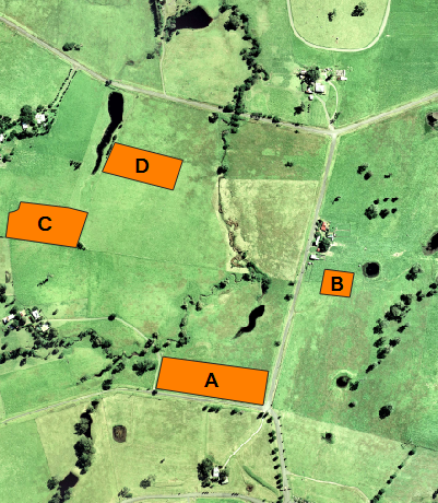
Material ID Paddock Name Area (ha) Animals 6 paddockA 1.5 23 Sheep, 7 Lambs 7 paddockB 0.3 2 Cows 8 paddockC 1.2 20 Sheep 9 paddockD 1 4 Cows, 2 Calves
- Set the pollutant export properties for material ID 1. This is the material ID for all areas within the model domain not covered by a material region. These pollutant export properties define the release and deposition of clay sediment. Sediment pollutants generally use the 'Shear1' method. For more information on 'Shear1', refer to Section 4.5.3.3.2 of the TUFLOW CATCH Manual.
- Set the pollutant export properties for material ID 4 (waterholes, eddies, etc). These properties define settling (deposition velocity) of alive and dead E. coli to 2 meters per day (approx 25cm during the simulation).
- Set the pollutant export properties for material ID's 6 (paddockA), 7 (paddockB), 8 (paddockC) and 9 (paddockD). These properties define the accumulation (rate) and washoff of alive and dead E. coli for the animals on the paddock.
- For this tutorial, leave all interventions commands as is. This section of the .tcc will be discussed in TUFLOW CATCH Tutorial 02.
- Save the .tcc.

Receiving Model (TUFLOW FV)
For this tutorial, leave all commands as is. This section of the .tcc will be populated in TUFLOW CATCH Tutorial 03.
Running the Simulation
- In Windows File Explorer, navigate to the TUFLOWCATCH\runs folder. The TUFLOW CATCH plugin created a batch file (.bat) that references the .tcc called Demonstration.bat.
- Save a copy of Demonstration.bat as _run_TC01_CATCH.bat and open the file in a text editor.
- Update the batch file to reference the TUFLOW CATCH executable:
set exe="..\..\..\..\exe\TUFLOWCATCH\2026.0.0\TUFLOWCATCH.exe"
%exe% TC01_001.tcc - Double click the batch file in file explorer to run the simulation.
Troubleshooting
See tips on common mistakes and troubleshooting steps if the model doesn't run:
Check Files and Results Output
Complete the steps outlined in the following links to review check files and simulation results from the TUFLOW CATCH pollutant export model simulation:
Reviewing Model Performance
There are a number of useful outputs from TUFLOW CATCH for reviewing the model performance.
TUFLOW CATCH Log File (.catchlog)
The first file to review is the TUFLOW CATCH Log File (.catchlog). The Log Folder == log command in the .tcc controls where the .catchlog is written.
Navigate to the Modelling\TUFLOWCATCH\runs\log folder and open the TC01_001.catchlog file in a text editor. It contains a summary of the TUFLOW CATCH simulation. The following are the key points to review:
- Global Settings: The commands from the 'Global Settings' section of the .tcc are echoed here. Review these to confirm that the correct settings have been applied.

- Simulation Configuration: The .catchlog outlines which models have been used and what simulation configuration has been run. In this tutorial, the catchment hydraulic and pollutant export models have been applied, indicating a pollutant export configuration.

- Run Status: At the end of the file, a message will confirm the simulation outcome.
- If successful, it will state 'Run Successful'
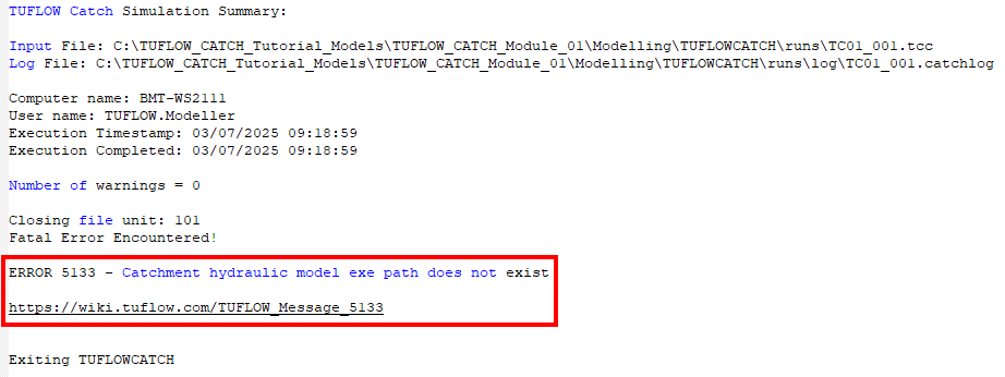
- If an issue occurred, the simulation will stop and an error message will be reported. An example error is shown in the image below.
- Note: Each TUFLOW CATCH error message has a corresponding wiki page that provides further details about the error, and suggestions for how to fix the issue. Refer to 5xxx Messages for a list of all TUFLOW CATCH related error messages.
- If successful, it will state 'Run Successful'


Other Log Files
Once the .catchlog has been reviewed, it is recommended to check the TUFLOW Log File (.tlf) if the catchment hydraulic model has been specified and to check the TUFLOW FV Log File (.log) if the receiving model has been specified. These files contain TUFLOW and TUFLOW FV specific check, warning and error messages.
TUFLOW Log File (.tlf)
Since the catchment hydraulic model is specified in this tutorial, review the TUFLOW Log File. The Log Folder == log command in the .tcc defines where the .tlf is written
Navigate to the Modelling\TUFLOWCATCH\runs\log folder and open the TC01_001_catchment_hydraulic.tlf file in a text editor.
- Scroll down to the bottom to 'Simulation Summary'. This includes information about the computation time, messages, volume calculations and mass error.
- Review any check, warning or error messages.
- For more information on reviewing TUFLOW log outputs, refer to HPC Model Review.
TUFLOW FV Log File (.log)
The receiving model has not been specified in this tutorial, so no TUFLOW FV Log File (.log) has been created. The TUFLOW FV Log File will be reviewed in TUFLOW CATCH Tutorial 03.
Conclusion
- A TUFLOW CATCH Pollutant Export model was created. A downstream receiving polygon was used to track pollutants in the receiving waters.
- Check files were used to review the transfer from the Catchment Hydraulic model (TUFLOW HPC) into the receiving polygon.
- TUFLOW CATCH time series results and TUFLOW map outputs were assessed to observe the pollutant behaviours.
- For further training opportunities see TUFLOW Training Catalogue and/or contact training@tuflow.com.
| Up |
|---|