Tutorial Module06 Archive

Introduction

Module 5 introduced a simple flood impact assessment to model and identify impacts resulting from a simple development. This module considers a scenario where the local Council rejected the proposed development because of the afflux generated in the area to the south (upstream) of the road crossing east to west. While the development proposal was rejected, the application did highlight to Council the lack of capacity of the bank of culverts and the relatively low flood immunity of the road crossing. In this module we investigate a simple upgrade of the structure through the use of a bridge to increase discharge capacity and improve the flood immunity. Module 5, including the creek as a 1D channel, forms the base model that we are going to use.

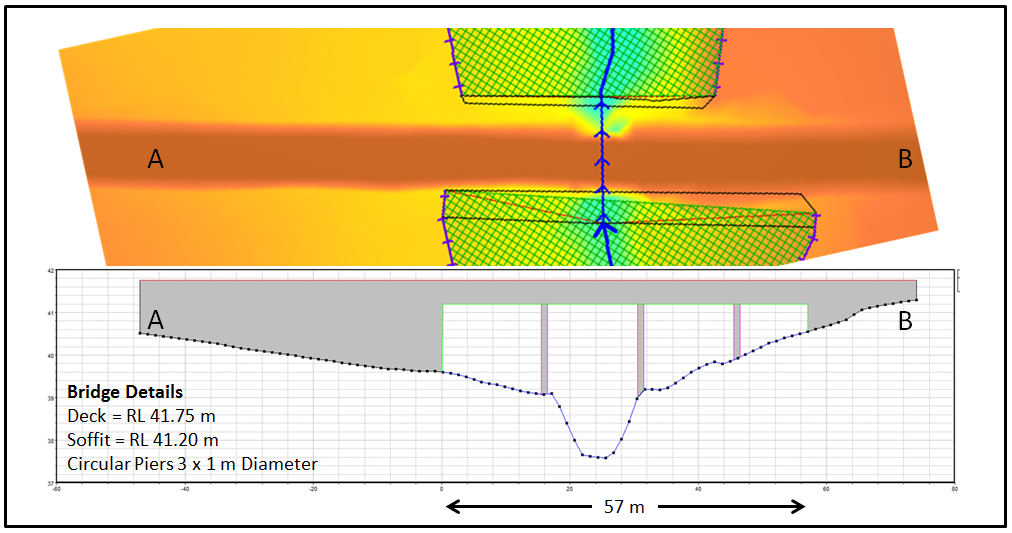
In this module we will model replacing the bank of culverts at the northern road crossing with a large bridge structure that spans the creek and part of the floodplain. The proposed bridge upgrade and key bridge details are presented in the simplified plan and section below. (Note that the plan view has been rotated slightly for visualisation purposes and the section is presented via the USACE program HECRAS.)

Using TUFLOW, bridges and large rectangular culverts can be modelled in either 1D, 2D or a combination of both 1D and 2D. This tutorial will show you how to setup a bridge using conventional low and high flow approaches with each of these 1D only , 2D only and 1D/2D combined methods. These include:

• Bridge Modelling Option 1: 1D Bridge with 2D Weir Overflow (1D/2D Combination)
• Bridge Modelling Option 2: 1D Bridge with 1D Weir Overflow (1D Only)
• Bridge Modelling Option 3: 2D Layered Flow Constriction (2D Only)

You will setup the files to run all three differing methods and then use the scenario features presented in Module 5 to select which bridge approach/s to model.




Modify GIS Files

We are testing a possible upgrade that replaces the bank of box culverts with a wide span bridge. The box culverts within the creek channel are therefore to be removed from the model and replaced by a cross section of the bridge. The road pavement is also to be regraded as part of the upgrade.

Revise the Road Crest

Currently a 2d_zsh layer (created in Module 3) is used to raise the zpts along the line and length of the northern road up to the road deck levels. This part of the tutorial will use 2d_zsh layers to regrade the road embankment. The road crest elevation will be amended and parts of the embankment lowered at the location of the 2D bridge. Follow the instructions at the relevant link below for your GIS package.

• MapInfo
• ArcGIS
• QGIS

Bridge Modelling Option 1: 1D Bridge with 2D Weir Overflow

For the first of our three bridge modelling techniques we will represent the flow area under the bridge up to the bridge soffit, the piers and energy losses through the structure using a 1D bridge channel. Bridge surcharge will be modelled in the 2D domain in a similar manner to the current 1D/2D culvert modelling approach. We have provided the required bridge cross section and bridge loss coefficient with height table (xs_bridge.csv and lc_bridge.csv respectively). Importantly, the highest elevation in the bridge cross-section is set at the soffit level of the bridge opening. The loss coefficient table defines the fraction of the kinetic energy (V²/2g) that is lost due to obstructions such as piers and the bridge deck. These loss coefficients have been developed with reference to the methods outlined Hydraulics of Bridge Waterways (Bradley, 1978). Open the csv files to understand how the bridge is modelled within TUFLOW (you may wish to produce a scatter plot of the cross section file to help visualise the bed profile). To update the model follow the instructions at the relevant link below for your GIS package.

• MapInfo
• ArcGIS
• QGIS

Bridge Modelling Option 2: 1D Bridge with 1D Weir Overflow

Using this approach we will use the 1D bridge section developed for Option 1 to represent the flow area under the bridge (as such please ensure you have completed Bridge Option 1). For this option, instead of using the 2D DEM to model bridge surcharge, we will create a 1D weir channel. This method requires us to modify a number of files including our 2D domain and 1D/2D boundary layers in the region between the cross sections immediately upstream and downstream of the structure. Follow the instructions at the relevant link below for your GIS package.

• MapInfo
• ArcGIS
• QGIS

Bridge Modelling Option 3: 2D Layered Flow Constriction

Finally, we can also model the obstruction and losses caused by the bridge in 2D only, using a layered flow constriction. We have provided the location of the layered flow constriction to be used to model the replacement bridge on the northern road. This data is in the Module Data folder under Module_Data\Module_06\2D_Bridge. Three GIS layers are provided: one with a polygon defining the 2D cells over which the flow constriction is to be applied, another containing height and depth points for the layers below and immediately above the bridge obvert and the third to lower the 2D grid cells at the bridge location. Follow the instructions at the relevant link below for your GIS package.

• MapInfo
• ArcGIS
• QGIS

For application of 2D layered flow constriction form losses, a handy reference is the Technical Memo on modelling bridge piers in 2D using TUFLOW available at: http://www.tuflow.com/Library.aspx?TechnicalDocuments

Modify Simulation Control Files and Set-up a TUFLOW Scenario

Now that we have made all of the necessary changes to the GIS layers, we need to update our control files to include the option of modelling the replacement bridge.

• MapInfo
• ArcGIS
• QGIS

Run the Simulation

Using your preferred method for starting TUFLOW, run the newly created M06_5m_~s1~_001.tcf. Please refer to Module 1 for a detailed description of the various methods for running a TUFLOW simulation.
In this tutorial we are using a batch file to run simulations. The use of an If Scenario requires a new -s1 switch to be added to the command line that launches the model simulation (shown in red below). TUFLOW replaces the s1 switch with the name of the scenario in all output files. Thus, the command line in our batch file looks like this:


set TUFLOWEXE=C:\TUFLOW\Releases\2017-09-AC\w64\TUFLOW_iSP_w64.exe set RUN=start "TUFLOW" /wait "%TUFLOWEXE%" -b %RUN% -s1 FINB1 M06_5m_~s1~_001.tcf %RUN% -s1 FINB2 M06_5m_~s1~_001.tcf %RUN% -s1 FINB3 M06_5m_~s1~_001.tcf

Try updating the batch file to simulate the EXG scenario. A second set of result and check files will be written with the name of all output files containing the s1 switch EXG. Also try to simulate the model with a scenario name of your choosing to try to trigger the error message Scenario not recognised.


If the model fails to start correctly please refer to the troubleshooting section at the end of this page.


Review Check Files

Once the model has started we can review the check files to ensure the changes have been correctly applied. From the TUFLOW\check\2d\ folder import (into MapInfo) or open (ArcMap and QGIS) the following check files:

Bridge Option 1

• check\2d\M06_5m_FINB1_001_zsh_zpt_check
• check\2d\M06_5m_FINB1_001_bcc_check
• check\1d\M06_5m_FINB1_001_nwk_C_check
• check\2d\M06_5m_FINB3_001_grd_check
  

Bridge Option 2

• check\2d\M06_5m_FINB2_001_zsh_zpt_check
• check\2d\M06_5m_FINB2_001_bcc_check
• check\1d\M06_5m_FINB2_001_nwk_C_check
• check\2d\M06_5m_FINB2_001_grd_check
  

Bridge Option 3

• M06_5m_FINB3_001_lfcsh_uvpt_check
• M06_5m_FINB3_001_grd_check
• M06_5m_FINB3_001_zsh_zpt_check
• M06_5m_FINB2_001_bcc_check

For both Bridge Modelling Options 1 and 2 at the location of the bridge you should see the 1d_nwk line representing the bridge. Viewing the attributes of the nwk_C_check layer should show the bridge (and weir for option 2) and its attributes (the replacement for the old bank of culverts). For Bridge Modelling Option 3 interrogation of the elevation attributes in the grd_check and zsh_zpt_check layers should show that the zpt and 2D cell elevations at the location of the 2D bridge have been lowered, removing the sections of embankment. Interrogation of the lfcsh_uvpt_check layer shows the applied losses at the u and v zpts (cell sides). The values for 'L1_FLC' and 'L2_FLC' in the check file are different then those specified in the 2d_lfcsh_M06_bridge_001.MIF / 2d_lfcsh_M06_bridge_R_001.SHP layer. This value has been calculated by multiplying the specified loss by the cell size and applying it to each of the u/v zpts falling within the lfcsh polygon.

Review the Results

Open the 2D results in your results viewer or import to your GIS package. You should see that where we have replaced a section of the road embankment west of the creek, 2D model cells now become wet and convey flow. The images below represent the peak depth and velocity for the three bridge modelling approaches (FINB1-FINB3 from left to right).



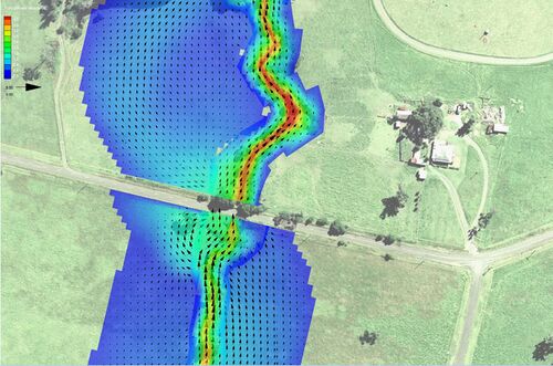
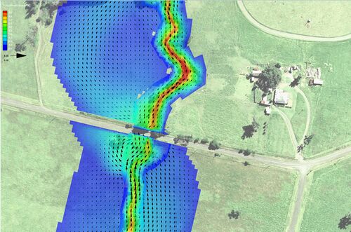
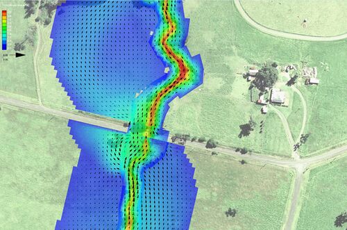
If you look at the 1D results (by importing the time series (_TS.mif or _TS_P.shp from the 1D results folder) you should see the new 1D bridge channel conveying flow. The peak water level at the upstream face of the bridge is about 40.9m. This compares with a peak water level in Module 4 of about 42.93m. Thus, in this instance the replacement bridge reduces the upstream face peak water level by approximately 2m (well we have put a very big bridge in there!!!!). Inspection of the results downstream of the bridge show that the increased conveyance also results in a slight increase in peak water level.

Extension - Test the Weirs and Multiply the Flow Rate

Following review of the results, it is clear that our bridge upgrade has had the desired effect in improving flood immunity of the road. To gain a better understanding of flows under an extreme event, we can re-run the models with an increased flowrate of 10 times the original.
Open the ..\bc_dbase\bc_dbase_M04.csv file in a text editor and modify the 'Mult Col 2' column as follows:


This will multiply the incoming flow rate by 10. For a descritption of the other attributes here, refer to table 4.28 of the 2010 TUFLOW manual
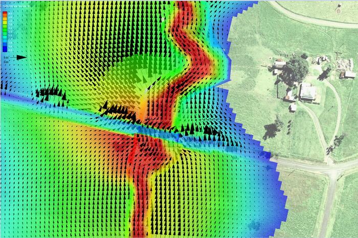
Re-run the model batch file and review the results and 1d_TS files. You should see that a significant component of the total flowrate now passes as weir flow across North Road for each of the three bridge modelling approaches. The following provides an example of this occuring for Bridge Modelling Approach 2:


Discussion on Differences Between Methods

We have tested three different methods to create a bridge within our model domain, each with a different 1D and/or 2D configurations. It's reasonable to ask - why would I want to know three different methods? When would I use the different methods in my own scenarios? Below is a few modelling aspects which you would take into account when considering how to schematise your bridge.


• Channel Schematisation
  Depending on how your channel is modelled, it is typically simpler and more stable to keep your inline structures in the same scheme. For example, if you had decided for model the creek in 1D, using a 1D bridge and Weir configuration would probably be a good choice.
• Weir Crest Shape
  Modelling the weir in 2D and keeping the bridge in 1D (as in option 1) is great for visualistaion, as it is possible to animate and show the road overtopping in 2D. However, this option is only really appropriate for when the weir crest is a simple shape. If the weir crest varies in height or has notches or steps, a 1D cross-section .csv file is more flexible and can more accurately define the topography.
• Cell Size
  The size of the structure relative to the 2D cell size can dictate which method is appropriate. If the cell size is too large to accurately represent the structure, 1D modelling techniques might be more appropriate.

Conclusion

We have used a TUFLOW If Scenario to replace the bank of culverts on the northern road crossing with a bridge that spans across the creek and part of the floodplain. We have investigated three conventional 1D/2D, 2D only and 1D bridge modelling approaches. The model has been structured such that we can remove the Bridge scenario from the model simulation and TUFLOW will revert to using the commands to run the 2D/1D model of Module 4 or the Development Scenario completed in Module 5. Use of the If Scenario command means that should you wish, many different scenarios can be easily simulated using the same geometry and control files (e.g. to test the impacts of multiple bridge options).

Congratulations!!! You have now completed Module 06.

Troubleshooting

If the TUFLOW simulation fails to start, TUFLOW will output the error in a number of locations. Firstly, check the Console Window or the TUFLOW Log File (.tlf) (located in the TUFLOW\runs\log\ folder with the name M06_5m_Bridge_001.tlf). This file can be opened in a text editor and the error is generally located at the end of the file. You can however search for "Error" if you cannot see the error. In most cases there is also a spatial location for the error message (if the error reported in the log file is prefixed by XY:). To check the location of the geographic errors, open the M06_5m_Bridge_001_messages.mif or M06_5m_Bridge_001_messages_P.shp file in your GIS package.

This section contains links to some possible problems that may occur when progressing through Module 6. If you experience a problem that is not detailed, please email support@tuflow.com or add and describe the problem on the discussion page.


• Save date of .tab file is later than .mif or .mid
• When reviewing check files, I can't see the changes
• ERROR 1025 - Number of bridge channels and BG tables not the same.
• CHECK 2210 - Top of first FC Layer is below ground level.
• Batch file does not run properly.




Advanced - HPC Solver (Optional)

This section will introduce how to run the model TUFLOW’s HPC (Heavily Parallelised Compute) solver, and how to fix some common issues that may occur when trying to run a simulation using Graphics Processing Unit (GPU) hardware.

TUFLOW HPC can run between 10 and 100 times faster than TUFLOW Classic using NVidia Graphics Processing Units (GPU)(depending on the model configuration and hardware performance).

Model Setup

To run the HPC solver using another .tcf file, simply perform the following steps:

1. Save the TUFLOW runfile (M06_5m_~s1~_001.tcf) as M06_5m_~s1~_002.tcf.
2. Add the following command to the TCF file:
   

   Solution Scheme == HPC ! Use HPC solver to run the model
   

3. If you have a CUDA enabled NVIDIA GPU device, you can also add the following command to run the HPC solver using GPU hardware:
   

   Hardware == GPU ! Run HPC solver on GPU
   

4. Update the batch file with the changes highlighted below in red.
   

   set TUFLOWEXE=C:\TUFLOW\Releases\2017-09-AC\w64\TUFLOW_iSP_w64.exe set RUN=start "TUFLOW" /wait "%TUFLOWEXE%" -b %RUN% -s1 FINB1 M06_5m_~s1~_001.tcf %RUN% -s1 FINB2 M06_5m_~s1~_001.tcf %RUN% -s1 FINB3 M06_5m_~s1~_001.tcf %RUN% -s1 FINB1 M06_5m_~s1~_002.tcf %RUN% -s1 FINB2 M06_5m_~s1~_002.tcf %RUN% -s1 FINB3 M06_5m_~s1~_002.tcf

5. Save the TCF file.
6. Run the TUFLOW Classic and HPC simulations.
7. Review the results.


TIP: To switch on the HPC solver via scenario control commands, please see the HPC Model Setup section of Module 5 (recommended).


Also, to learn how to optimise a HPC simulation to achieve the fastest simulation speed please complete Tutorial Module 2 and Tutorial Module 3


Results

Using the methods described above in the Viewing Results section of Module 1.

• Check the simulation logs in the DOS window, .tlf and .hpc.tlf log files.
• View the results in your preferred package.

Do the logs and results appear different to the TUFLOW Classic simulation?

Troubleshooting for GPU Simulations

If you receive the following error when trying to run the TUFLOW HPC model using GPU hardware:

TUFLOW GPU: Interrogating CUDA enabled GPUs … 
TUFLOW GPU: Error: Non-CUDA Success Code returned 

or

ERROR 2785 - No GPU devices found, enabled or compatible.

Please try the following steps:

1. Check if your GPU card is an NVIDIA GPU card. Currently, TUFLOW does not run on AMD type GPU.
2. Check if your NVIDIA GPU card is CUDA enabled and whether the latest drivers are installed. Please see GPU Setup.


If you experience an issue that is not detailed above please send an email to support@tuflow.com