Tutorial Module01 Archive
- TUFLOW Simulation Control File (TCF)
- TUFLOW Geometry Control File (TGC)
- TUFLOW Boundary Control File (TBC)
- TUFLOW Boundary Condition Database (.csv)
- TUFLOW Materials File (.csv)
- 2d_bc_: A GIS layer defining the locations of external 2D boundaries.
- 2d_sa_: A GIS layer to define internal 2D flow boundaries.
- 2d_code_: A GIS layer containing polygons that define the cell codes (active or inactive status).
- 2d_loc_: A GIS layer defining the origin and orientation of the 2D grid.
- 2d_mat_: A GIS layer defining the land-use (material) types within the 2D study area.
- *.asc: A DEM dataset defining the ground elevations within the 2D study area.
- Set up the model directory and sub-directories as recommended in the list below (for a more detailed description, please refer to the TUFLOW Manual). Alternatively, you can copy the TUFLOW folder and all sub-folders from the TUFLOW Folders Template folder in the supplied files to a local drive on your computer.
* If using SMS, the folder structure listed above is automatically created before running the model using the "Export TUFLOW files" command (see Run TUFLOW from within SMS).
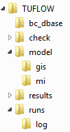
Sub-Folder Input / Output Description bc_dbase Input Boundary condition database(s) and input time-series data check Output GIS and other check files to carry out quality control checks (use Write Check Files). model Input Geometry (.tgc), Boundary (.tbc) and other model control text files (i.e. no GIS files). model\gis Input GIS layers that are inputs to the 2D and 1D model domains are contained within this folder: model\gis\ is typically used for all ArcGIS and QGIS files model\mi Input GIS layers that are inputs to the 2D and 1D model domains are contained within this folder: model\mi\ is typically used for MapInfo formatted GIS files results Output TUFLOW will output the results to this folder in a variety of formats as specified by the user. runs Input TUFLOW Control Files (.tcf) runs\log Output TUFLOW log files (.tlf) and messages layers.
The following points on TUFLOW folders and filenames are worth noting:
- * TUFLOW accepts any folder structure, though the above listed format is most commonly used and is recommended.
- * Whilst TUFLOW readily accepts spaces and special characters (such as ! or #) in filenames and paths, other software may have issues with these. It is therefore recommended that spaces and other special characters (such as dashes) are not used in the simulation path and filenames (without prior testing).
- * Folder paths, filenames, file extensions and TUFLOW commands are not case sensitive in any TUFLOW control files.
- * The model\mi\ is used for MapInfo inputs, model\gis\ for ArcGIS and QGIS inputs. Any directories that don't apply can be omitted, for example if you are working in MapInfo the model\gis directory may not be be required.
- * For ArcMap 10.1 and newer users, the ArcTUFLOW Toolbox can be used to automatically create the model folders, model projection, TUFLOW control files and run TUFLOW to create the template files.
- * For QGIS users, the TUFLOW QGIS Plugin can be used for the same tasks listed for the ArcTUFLOW toolbox.
- * TUFLOW accepts any folder structure, though the above listed format is most commonly used and is recommended.
- An aerial photo and DEM of the model area are provided. Open the following layers in your GIS software:
- Module_Data\Aerial_Photos\Aerial_Photo_M01
- Module_Data\DEMs\DEM_M01
- Create a projection file and write the template GIS files (to be used to build the model) for the project. For a description on how to do this please select your GIS package below.
- ArcGIS - Create Projection (not using the ArcTUFLOW Toolbox)
- Mapinfo - Create Projection
- QGIS - Create Projection (not using the QGIS TUFLOW Plugin)
- SMS - Create Projection and GIS Empty Files
- The next step is to create a TUFLOW Control File (TCF files are used to control the input and output from TUFLOW) and create the 'template' or 'empty' GIS files. TUFLOW will assign the same projection as the GIS layer created above to the template files and also set the file fields or attributes so they are compatible with the desired purpose of the file. See Empty Template GIS Files for more information about each of the TUFLOW template GIS files. In a text editor, create a new file and save to the TUFLOW\runs folder. Since this is Module 1 and the model we’ll produce has a 5m grid, name the file M01_5m_001.tcf.
- Enter the text as shown below into the newly created text file M01_5m_001.tcf:
Tutorial Model == ON
MapInfo Users:
GIS Format == MIF
MI Projection == ..\model\mi\Projection.mif
Write Empty MI Files == ..\model\mi\empty
ArcGIS and QGIS Users:
GIS Format == SHP
SHP Projection == ..\model\gis\Projection.prj
Write Empty GIS Files == ..\model\gis\empty | SHP
- Save the TCF file.
Note:
* You can insert comments into this file if you find it helpful. This is highly recommended. Comments are preceded by an exclamation mark or a hash symbol (i.e. ! or #). Comments can be written after the command or have their own line. Any command following the comment symbol is ignored by TUFLOW.
* Notice the syntax highlighting in the commands listed above. If you have not already enabled syntax highlighting in your preferred text editing software, we recommend you do. Instructions are provided in the Tips and Tricks section for each software Notepad++, UltraEdit, TextPad. - Running TUFLOW from a Batch-file (recommended for this tutorial)
- Running TUFLOW from UltraEdit
- Running TUFLOW from Notepad++
- Running TUFLOW from Right Click in Windows XP
- Running TUFLOW from Right Click in Windows 7
- Running TUFLOW using SMS
- Start TUFLOW from a batch file using the TCF file we have created (M01_5m_001.tcf). Follow the steps outlined in, Running TUFLOW from a Batch-file to create the batch file.
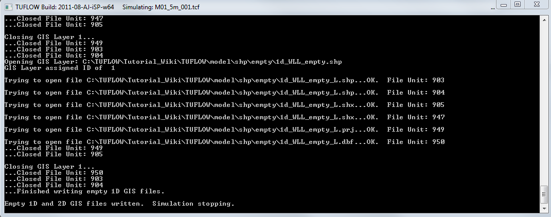
- Double click the created batch file (.bat) from Windows Explorer to execute the simulation. A console window should appear as shown below:
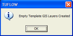
- After a few seconds the information dialog box shown below should appear. Click OK to close the windows.
- Check the folder specified to view the ‘Empty’ template files have been written.
- For MapInfo Users these should be in TUFLOW\model\mi\empty\
- For ArcGIS and QGIS Users this should be TUFLOW\model\gis\empty\
- 12D TIN (Module_Data\DEMs\DEM_M01.12da)
- SMS TIN (Module_Data\DEMs\DEM_M01.SMS.tin)
- Vertical Mapper Grid (Module_Data\DEMs\DEM_M01.tab and .grd files)
- Arc Spatial Analyst format (.img)
- Specifying origin coordinates and a second set of coordinates for a point along the X-axis of the domain;
- Digitising a line to represent the bottom edge of the 2D domain (with the line starting at the origin and finishing at a secondary location along the X-axis; or
- Specifying the origin coordinate and domain orientation angle.
- Create a new text file called M01_5m_002.tgc. Save the file in TUFLOW\model\ folder. This file will become our TUFLOW Geometry Control File (TGC).
Notice this time we’ve used ‘002’ for numbering the file. This is part of a sound naming convention. This TGC file will be used for simulation ‘002’, hence we’ll number the TGC and any new GIS layers that are added during this model iteration with the same number. This way, in the future, we’ll know that this file and any new tables were created for simulation ‘002’. This also allows us to revert to a previous version of the model without have to undo any changes to the control or GIS files.
- We need to specify the location and dimensions of the TUFLOW domain (computational area) and also the cell size in the TGC file. Add the following text to the TGC file and save.
Note: you do not need to add the comments, but it is a good habit to get into
Origin == 292725, 6177615 ! bottom left corner of grid
Orientation == 293580, 6177415 ! another point along the x-axis of the grid
Cell Size == 5 ! cell size in metres
Grid Size (X,Y) == 850, 1000 ! grid dimensions in metres
- For instructions on how to complete these steps using SMS, see Define the 2D Domain using SMS.
- Speed, direct input of the DEM to TUFLOW is very fast compared to a point inspection in a GIS software; and
- Flexibility, if the cell size, dimension or rotation of the TUFLOW model is changed, TUFLOW will update the elevations automatically.
- Firstly, add the Set Code == 0 command to the TGC file. This sets all 2D cells to inactive, we will next define the active areas in GIS.
- To set the active areas please select you GIS package below:
- Define active area in Mapinfo
- Define active area in ArcGIS (arcTUFLOW)
- Define active area in QGIS
- Define active area in SMS
- Open M01_5m_001.tcf in your text editor and save a copy as M01_5m_002.tcf.
- Comment out (or delete) the "Write Empty GIS Files" line, using a comment character (! or #)
- ! Write Empty GIS Files == ..\model\gis\empty
- ! Write Empty GIS Files == ..\model\gis\empty
- Add the following commands (to the M01_5m_002.tcf file) and save the file.
- Geometry Control File == ..\model\M01_5m_002.tgc
- Read Materials File == ..\model\materials.csv ! This provides the link between the material ID defined in the .tgc and the Manning's roughess
- Geometry Control File == ..\model\M01_5m_002.tgc
- Upstream and downstream flow boundaries
- Downstream water level boundaries
- Water sources and abstractions
- Direct rainfall or infiltration
- 1D/2D and 2D/2D links
- A flow vs time (QT) boundary and a source-area (SA) boundary will be used as inflows.
- A stage vs discharge (HQ) boundary is used for the outflow.
- Create a new text file and save as M01_5m_002.tbc in the TUFLOW\model folder. This is our TUFLOW Boundary Condition File.
- Open this file in a text editor and add the following lines of text and save.
MapInfo Users
Read GIS BC == mi\2d_bc_M01_002.mif
Read GIS SA == mi\2d_sa_M01_002.mif
ArcGIS or QGIS Users
Read GIS BC == gis\2d_bc_M01_002_L.shp
Read GIS SA == gis\2d_sa_M01_002_R.shp
- The process for adding the TUFLOW utilities to Excel is detailed here: Excel Tips.
- alternatively, to use the macro without adding them to Excel, simply open the TUFLOW_Tools_v2.0.xlam in the Module_Data\Module_01\Excel folder.
- To create a bc_dbase, start by copying the template bc database (TUFLOW Tutorial Model BC Database.xls) from the Module_Data\Module_01\Excel folder into the TUFLOW\bc_dbase folder (keep the same file name). Open the file in Excel by double clicking on it in Windows Explorer.
You’ll notice that there are two worksheets. Firstly we’ll complete the bc_dbase worksheet which has column headers in the first 9 columns. As we fill in the entries, it should become clear how they are used, and how TUFLOW interprets the data.
- Enter the name of the first upstream boundary condition into cell A2. The name must appear exactly as it does in the 2d_bc_M01_002 layer, (i.e. FC01).
- Enter the text “100yr2hr.csv” into cell B2 as per below.
- Enter the text “inflow_time_hr” into Cell C2 and “inflow_FC01” into Cells D2 as shown below, leaving the remaining 5 columns blank.
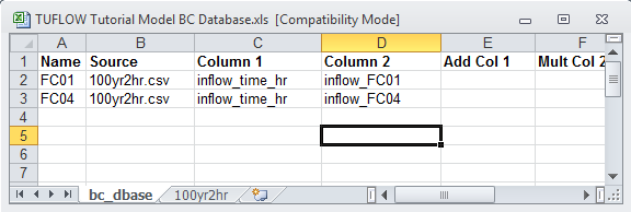
Name Source Column 1 Column 2 FC01 100yr2hr.csv inflow_time_hr inflow_FC01 FC04 100yr2hr.csv inflow_time_hr inflow_FC04
For each of the inflow boundaries, we have specified the GIS name in the name column, specified a source file for TUFLOW to extract the time series data (100yr2hr.csv) and specified the data columns, corresponding to the data headers in the source timeseries file.
- In Excel, switch to the 100yr2hr sheet, and review the hydrographs that have been provided. Note at the stage the "Inflow_FC02" hydrograph is not being used.
- If you haven't already, open the TUFLOW_tools_v2.0.xlam, this should create a new drop Menu Item titled TUFLOW. Navigate to this window and select Entire Worksheet to csv.
TUFLOW Tools for Excel
This utility saves each sheet in the workbook as a .csv file and uses the sheet name to set the filename. If you look in the TUFLOW\bc_dbase\ directory, there should be two new files, "bc_dbase.csv" and "100yr2hr.csv". This has saved all of tabular data from these sheets into a format that TUFLOW can read. The .csv file is a simple text file, with data separated by a comma. This is shown in a text editor below.
Note: The 100yr2hr worksheet had a chart in excel, this can not be stored in .csv format and is omitted.
- Open M01_5m_002.tcf in your text editor and make the following edits.
- Add the following commands (to the M01_5m_002.tcf file) and save the file.
BC Control File == ..\model\M01_5m_002.tbc
BC Database == ..\bc_dbase\bc_dbase.csv
- Open M01_5m_002.tcf in your text editor and make the following edits.
- Add the following commands and save the file.
- Start Time == 0 ! Start Simulation a 0 hours
- End Time == 3 ! End Simulation a 3 hours
- Timestep == 1.5 ! Use a 2D timestep of 1.5 seconds
- Log Folder == Log ! Redirects log output (e.g. .tlf and _messages GIS layers to the folder "log"
- Output Folder == ..\results\M01\2d\ ! Redirects results files to TUFLOW\Results\M01\2d\
- Write Check Files == ..\check\2d\ ! Specifies check files to be witten to TUFLOW\check\2d\
- Map Output Data Types == h v q d MB1 MB2 ! Output: Levels, Velocities, Unit Flows, Depths, Mass Error
- Map Output Interval == 300 ! Output every 300 seconds (5 minutes)
- Store Maximums and Minimums == ON MAXIMUMS ONLY ! Save peaks values
- Map Output Format == GRID DAT ! Output directly to GIS (grid) as well as SMS (dat) format
The final command "Map Output Format" controls the output file format, this is discussed further in the results viewing section below.
The TUFLOW simulation is now ready to be run for the first time. - Start Time == 0 ! Start Simulation a 0 hours
- GIS Grid format: Output directly to raster grid format suitable for use in most GIS packages.
- Can be output in ESRI ascii (.asc) format with the TUFLOW Control File command is: Map Output Format == ASC. This is recommended for MapInfo / Vertical Mapper users.
- Can be output in ESRI binary float (.flt) format with the TUFLOW Control File command is: Map Output Format == FLT. This is recommended for ArcMap and QGIS users.
- SMS .dat format: Used by SMS and also by the QGIS TUFLOW Plugin (both methods outlined below). TUFLOW Control File command is: Map Output Format == Dat
- SMS .xmdf format: Used by SMS and QGIS TUFLOW Plugin. It's a more advanced version of the .dat above. It contains all results in a single output file. The TUFLOW Control File command is: Map Output Format == XMDF
- WaterRide .wrb format: Used by Waterride. The TUFLOW Control File command is: Map Output Format == WRB
- BlueKenue .t3 format: Used by BlueKenue. The TUFLOW Control File command is: Map Output Format == T3
- In Windows Explorer, navigate to the TUFLOW\runs\Log\ directory and locate the M01_5m_002.tlf file. Open this file into your text editor. At the end of this file is the Simulation Summary. As the name suggest this contains a summary of the TUFLOW simulation performance. The first part of the summary contains some information about the files, times and computation time.
- Open the M01_5m_002_messages.csv file in the TUFLOW\runs\log\ directory. It provides a summary of the messages. For example:
- To view the location of this error, import the M01_5m_002_messages.mif or M01_5m_002_messages_P.shp file into your GIS package.
- In the simulation summary of the .tlf file (see above)
- In the _ TUFLOW Simulations.log, this is written to the TUFLOW\runs\ directory.
- This is a text file that can be opened in your text editor. For the M01_5m_002 that was just simulated, here is an extract.
Finished: M01_5m_002 fCME = -2.03% pCME = -2.03%
- The _ TUFLOW Simulations.log also contains a variety of other information, such as date, computer name, TUFLOW build version, the CPU hours and a other useful data.
- Time-series mass balance output. This is written to the same location as the 2D model results (in this case TUFLOW\results\M01\2d\). This file has the same name as the runfile (TCF) with the suffix, _MB.csv. As such the mass balance spreadsheet for this simulation is called M01_5m_002_MB.csv. Open the file in Excel. It contains a summary of the mass entering and leaving the model. Plot the first (time) and last (cumulative mass error %) columns within the spreadsheet to review the time varying mass error values.
- MB1 and MB2 map output. These 2D map outputs can be viewed using the methods described above in Viewing Results.
- Save date of .tab file is later than .mif or .mid
- ERROR 2014 - No active cells within SA inflow polygon
- Why does the TUFLOW console window open, though the TCF isn’t read and the simulation doesn’t execute?
- Save the TUFLOW runfile (M01_5m_002.tcf) as M01_2p5m_003.tcf
- Save the geometry control file (M01_5m_002.tgc) as M01_2p5m_003.tgc (don't forget to update the .tcf, to include the new geometry control file).
- Modify the cell size in the geometry control file.
- Reduce the timestep in the .tcf from 1.5 seconds to 0.5 second:
- Timestep == 0.5 ! Use a 2D timestep of 0.5 seconds
- Timestep == 0.5 ! Use a 2D timestep of 0.5 seconds
- Run the model.
- For instructions on how to complete these steps using SMS, see Change Cell Size Using SMS.
- Save the TUFLOW runfile (M01_2p5m_003.tcf) as M01_2p5m_004.tcf.
- Add the following command to the TCF file:
- Solution Scheme == HPC ! Use HPC solver to run the model
- Solution Scheme == HPC ! Use HPC solver to run the model
- If you have a CUDA enabled NVIDIA GPU device, you can also add the following command to run the HPC solver using GPU hardware:
- Hardware == GPU ! Run HPC solver on GPU
- Hardware == GPU ! Run HPC solver on GPU
- Save the TCF file and run the model.
- For instructions on how to complete these steps using SMS, see TUFLOW HPC Using SMS.
- Check the simulation logs in the console window, .tlf and .hpc.tlf log files.
- View the results in your preferred package.
- Check if your GPU card is an NVIDIA GPU card. Currently, TUFLOW does not run on AMD type GPU.
- Check if your NVIDIA GPU card is CUDA enabled and whether the latest drivers are installed. Please see GPU Setup.
Introduction
Please read the Tutorial Model Introduction before starting this tutorial. It outlines the programs requiring installation and where the source data can be downloaded (e.g. aerial photos, DEM...).
In this first module, a fully two-dimensional (2D) model is built. The steps required to build, run and review a basic 2D TUFLOW model are listed in the table of contents above and shown in the workflow diagram below.

Throughout the tutorial we will create and describe a number of TUFLOW Control Files and GIS layers that are used as input to a TUFLOW model. The TUFLOW Control (text) files introduced in this tutorial include:
The Geographic Information System (GIS) layers used in this tutorial are:
Project Initialisation
Setup Model Folders
TUFLOW models are separated into a series of folders which contain the input and output files.

Set GIS Projection and Create Empty (Template) GIS Files
The first step when creating a TUFLOW model always requires the user to define the GIS projection (i.e. the geographic coordinate system to be used for the TUFLOW model) and also write template GIS files for future model inputs.
Note: All model inputs will need to use a common projection.
Run TUFLOW to Create Empty (Template) GIS Files
We now need to run TUFLOW using the TUFLOW Control File (TCF). There are a number of ways TUFLOW can be setup to run. In each case the TUFLOW executable is started with the TCF as the input. For more information on running TUFLOW please refer to the TUFLOW Manual. The most common ways are outlined below. We will be using a batch file for this tutorial, however any of the methods below will work.


TUFLOW Geometry Control File (TGC) Inputs
Define Location and Dimensions of the 2D Domain
Pre-processing of the Digital Elevation Model (DEM) is not covered in this tutorial. The DEM for the tutorial is provided in a variety of formats, including:
Defining the location and orientation of the TUFLOW 2D domain can be undertaken using three different methods as follows:
The first method is covered in this tutorial. It is required if using an unlicensed version of TUFLOW. The second method is the most commonly used method on day to day projects.
ArcGIS, Mapinfo, and QGIS Users:
SMS Users:
Define Elevations
In the previous section, the extent and dimensions of the 2D domain were defined. We now need to assign elevations at each 2D cell centre, mid-side and corner. These points are known as Zpts.
Knowledge of 2D domain geometry is fundamental to understanding how TUFLOW works. A brief description on the computational function of each of the Zpts in a TUFLOW cell is given in the Zpt Description page.
There are two methods to assign the elevations to the Zpts. The first is to directly input the elevation model into TUFLOW as either a TIN or gridded DEM dataset. TUFLOW will assign the elevations from the elevation dataset to Zpts within the DEM / TIN. This offers the following benefits:
The second approach is to manually assign the elevation at each of the points using a GIS package. This approach involves TUFLOW writing out the Zpt layer in GIS format and the user defining the elevation at each point in a GIS package. For earlier versions of TUFLOW this method was the only option, it has largely been superseded, but is still supported. For the reasons listed above direct input of the elevation model as either a TIN or DEM is the preferred approach.
ArcGIS, Mapinfo, and QGIS Users
The process of using a direct TIN or DEM read into TUFLOW is outlined below. It is recommended that you have the DEM open in your GIS package, if you do not have it open it can be found in the Module_Data\DEMs\ folder under your GIS package name. Please select one of the following approaches, for users without 12D or SMS the DEM method is recommended.
SMS Users
The model elevations were previously defined during the Define 2D Domain Using SMS) step. No furtyher actions are required. Please progress to the next step.
Define Preliminary Active and Inactive Areas of the 2D Domain
By default, every grid cell in a TUFLOW model will set as active, thus TUFLOW will allow water to flow anywhere within the extents of the 2D domain. It is rare for a catchment to be a perfect rectangle! To reduce output file sizes and run times, permanently dry and inactive areas can be removed from the model. This can be an iterative process, you might run the model initially and refine. For the purpose of the tutorial you are provided with a polygon, which we will use to define the active area in your GIS package.
Discussion on Command Order
When developing a TUFLOW model, it is important to consider how TUFLOW interprets each command in the control files (TCF, TGC, TBC, ECF etc.). In most cases, the location or order within the file is not important, with the last occurrence of that command prevailing. However, for certain commands, particularly those in the TGC file, the order is critical. TUFLOW uses data layering protocol in the TGC.
Commands in the TGC file are read sequentially from the top of the file to the bottom. Where commands alter details for a common cell location (such as code value, elevation or landuse specification), the cell value will be defined by the values specified by the file lower in the TGC. For example, in the case of the Read GIS Code command discussed in the previous section, the 2D cells that fall within the polygon in 2d_Code_M01_002 will define the active/inactive code status irrespective of any code values assigned by previous global code command Set Code == 0 command. Consider the following two blocks of "code" commands below:
Correct Order
Set Code == 0 ! this sets all cells to be inactive
Read GIS Code == ..\model\mi\2d_code_M01_002.MIF ! this updates the cells within the polygon to be active
This command order will achieve the desired outcome. We have initialised the code status for the entire model (as inactive), then updated the status (to active) in the areas contained within the GIS polygon.
Incorrect Order
This is an example of incorrect command order:
Read GIS Code == ..\model\mi\2d_code_M01_002.MIF ! this sets the cells within the polygon to be active
Set Code == 0 ! this sets all cells to be inactive
The second command which sets all cells to be inactive, overwrites the values read in from the GIS layer. The end result will be no active cells in the TUFLOW model!
Define the Materials (Surface Roughness)
Surface roughness or bed resistance values (e.g. Manning’s n) are assigned to Materials values. The Module_Data\Module_01\ folder already contains the materials table that we’ll use. We will review these in a GIS package, please select one of:
In order for TUFLOW to associate the Manning’s n to the Material ID, a TUFLOW Materials File is required. This is can be either a text file (.tmf) or an .csv file which can be edited in Excel. In this tutorial model we will utilise the second (.csv) option.
As a minimum this file must contain two columns; the first being the Material ID (as specified in the GIS layer), and the second being the Manning’s n. The .csv file for this tutorial has already been created. Additional data such as loss parameters (applicable for direct rainfall modelling) and depth varying Manning's n values are covered in later modules. The .csv file is presented below (viewed in Excel).

Copy the materials.csv file from the Module_Data\Module_01\Text\ folder into the TUFLOW\model folder.
TUFLOW uses this file to apply the surface roughness values to the 2D cells based on the 2D cell Material values as defined by the Set Mat and Read GIS Mat commands. This materials files will be referred to in the .tcf when we modify this later.
TUFLOW Control File (TCF) Updates
The final step in setting the model geometry is to update our TUFLOW Control File (TCF) to point to the new TUFLOW Geometry Control (TGC) and TUFLOW Materials File (TMF).
TUFLOW Boundary Condition Control File (TBC) Inputs
In this step we introduce the TUFLOW Boundary Condition Control File (TBC) and Boundary Condition Database (bc_dbase). The TBC file contains information regarding the location of boundary conditions and internal links within the model. These include, but are not limited to:
Define Boundary Condition GIS Locations
For this step, upstream and downstream boundaries are applied.
For details on setting up the GIS layers required, please select your GIS package.
TUFLOW Boundary Control File (TBC) Updates
We next need to read the GIS files created above into the TUFLOW model. We need to create a new text format control file which is the TUFLOW Boundary Condition (TBC) this is similar to the TGC in that it contains the links with the GIS layers.
TUFLOW Boundary Condition Database (bc_dbase)
We now need to associate a hydrograph with each of the upstream boundaries. This is carried out using a boundary condition database. The boundary condition database (bc_dbase) is a powerful function of TUFLOW, potentially saving hours of data input that might otherwise be necessary. The bc database is a comma delimited file with a CSV extension. It can be opened in Excel or any text-editing program. The best approach for managing boundary data is to use an Excel spreadsheet and export the CSV files using the “Save csv” tool provided in the TUFLOW Tools Macro for Excel.
Follow the below listed steps:


TUFLOW Control File (TCF) Updates
The final step in setting the boundaries is to update our TUFLOW Control File (TCF) to point to the new boundary files (TBC and bc_dbase.csv).
TUFLOW Simulation Control File (TCF) Updates
Set Model Controls
This is the last step before running the simulation. Once this step has been completed, most of the groundwork has been completed. Subsequent modules build upon this base.
Run Simulation
Using your preferred method start your TUFLOW simulation. We recommend using the batch file approach, see Running TUFLOW from a Batch-file.
The simulation will take a few minutes to process (depending on the speed of you computer). While the modelling is running, it is worth filling out your Modelling Log. a modelling log includes developer notes keeping a record of TUFLOW simulations and changes from one version to the next. This is not detailed in the Tutorial model but is good practise to get in to. A modelling log is discussed here: TUFLOW Modelling Log (this link was on the tutorial model introduction page). A template modelling log is included in the TUFLOW Folders Template\TUFLOW\ folder of the files supplied with this tutorial.
If your simulation has been successful, the console window should look like the image below.
For instructions on how to complete these steps using SMS, see Set Model Controls and Run the Simulation using SMS.

Viewing Results
Output Formats
In this section we will look at viewing the 2D results. There are a variety of options for viewing TUFLOW results. The following options are most commonly used:
It is also possible to get multiple outputs for a single simulation. For example, GIS grid and WaterRide output can be written using teh syntax Map Output Format == FLT WRB
Note: Prior to the 2013 release of TUFLOW, it was necessary to use a freely available utility (called TUFLOW_to_gis.exe) to convert the .dat or .xmdf formats to GIS grids. However, it is now possible to have TUFLOW output the results directly to GIS format. The .flt format is the default for the 2013-12-AB version and this is best when using ArcMap or QGIS. However, if using MapInfo and Vertical Mapper the .asc format is required.
Depending on the software you are going to use to view the results, you may need to change the Map Output Format and Grid Format commands in the control file and re-run the model. For example if using SMS and ArcMap the recommended settings would be:
Map Output Format == XMDF FLT
However, if using WaterRide and Mapinfo the recommended settings would be:
Map Output Format == WRB ASC
It is also possible to control the frequency and output types for each output format separately, however this is not covered in this tutorial.
Viewing Results
Open and view the TUFLOW results in your viewing package, for instructions on this please select your results package below.
Reviewing Model Performance
When reviewing our model performance there are a number of useful outputs from TUFLOW. In this section we will introduce some of the available simulation check files and also review the stability and performance of the model. We will look at a number of GIS and text based outputs in this review.
Simulation Check Files
With the Write Check Files command specified in the TCF, TUFLOW will write a series of check files prior to the simulation starting. The check files are useful for reviewing the inputs have been correctly specified. This is particularly the case of long simulations, for example if you have a large model that runs for 12 hours and you are running a model with additional breakline (see Module 3), it is good to check that these features are correctly represented. This can be done using the check files whilst the 12 hour simulation is running, rather than waiting until the simulation finishes! We will introduce the check files as we progress with the tutorial modules. In the first module we will use the _zpt_check file, which contains all the final Zpt elevations, for the active model area. Please select your GIS package.
For information on other TUFLOW check files please refer to the Check Files page of the TUFLOW Wiki.
TUFLOW Log file
The first place to look is at the final output in the console window. If you missed this, for example if the model was run in batch mode this information is contained in the TUFLOW Log File (.tlf). Earlier on we add the following command to the TCF:
Log Folder == Log
This command controls where the log file is written. By setting this to Log it will be written to a Log directory under the runs directory.
SIMULATION SUMMARY

Input File: C:\TUFLOW\Tutorial_Wiki\TUFLOW\runs\M01_5m_002.tcf
Log File: C:\TUFLOW\Tutorial_Wiki\TUFLOW\runs\log\M01_5m_002.tlf

Start Time (h): 0.
End Time (h):   3.
Computational Steps (based on largest 2D timestep): 7200

CPU Time (hh:mm:ss):        0:01:08 [0.01891 hours]
Clock Time (hh:mm:ss):      0:01:14 [0202056 hours]

Simulation FINISHED
The next part of the Simulation Summary contains information on the messages issued by TUFLOW. Of note is the 2D Negative Depths (1). This indicates that the numerical solution has "overshot" and calculated a negative depth. Repeated negative depths are an indication that the model is not performing well. We will look at where these occur in the next section.
Total 1D Negative Depths: 0
Total 2D Negative Depths: 118

WARNINGs prior to simulation:     2  [1 not in _messages layer]
WARNINGs during simulation:     118  [0 not in _messages layer]
CHECKs prior to simulation:       0  [0 not in _messages layer]
CHECKs during simulation:         0  [0 not in _messages layer]
Following the messages section is a summary of the volumes and mass error in the model. The table towards the end shows the Peak Cumulative ME: was -1.19% and that this occurred at 0.27 hours into the simulation (16 minutes). It is preferable to have a Peak Cumulative ME below 1%. In the sections below we we look at determining where the mass error is occurring.
Peak Flow In (m3/s):   105.9 at Time 0.92
Peak Flow Out (m3/s):  84.1 at Time 1.21
Volume at Start (m3):  237
Volume at End (m3):    149824
Total Volume In (m3):  408904
Total Volume Out (m3): 246025
Volume Error (m3):     -13292 or -2.0% of Volume In + Out
Final Cumulative ME:   -2.03%

                                    Whole Simulation            Qi+Qo > 5%
Peak +ve dV (m3):                  160.0 at    0.89h       160.0 at    0.89h
Peak -ve dV (m3):                  -28.3 at    1.58h       -28.3 at    1.58h
Peak ddV over one timestep:        -12.0 at    0.89h        12.0 at    0.89h
Peak ddV as a % of peak dV:          7.5%                    7.5%
Peak Cumulative ME:               -2.03% at    3.00h      -2.03% at    3.00h
TUFLOW Messages Layers
TUFLOW writes a number of messages, in increasing order of severity these are: Check --> Warning --> Error. Each of the messages generated by TUFLOW has a four digit ID code. A description of each of these messages is given in the message database section of this wiki: (TUFLOW Messages Database). When a numerical model such as TUFLOW struggles to converge to a solution, spurious results such as negative depths can be generated. When this occurs TUFLOW creates a warning and writes this to the _messages.csv file and also to a GIS file. This can be opened in excel, or your GIS package.
| 2991 | 2 | 293285.826 | 6177861.233 | "WARNING 2991 - Negative U depth at [074;098]." | "Time = 0:38:33" | "Depth = -0.2" | "2D Domain = Domain_001" |
This may vary slightly or may not be there at all, depending on the version of TUFLOW you run.
This message indicates that Warning Message 2991 occurred during the simulation.

It can be seen that the warning message is occurring in the steep area of the creek bank.
Mass Balance Outputs
Mass balance can be an issue for badly configured numerical models (not just TUFLOW). A modeller should be aware of the health of the model to ensure that the model is well conditioned.
TUFLOW outputs the mass balance in a number of ways:
The MB1 output tracks the convergence of the solution at each cell since the previous output time. The MB2 is the cumulative sum of the MB1 output. In the image below the MB2 output is shown at the final timestep (3 hours). It highlights areas in which the 2D solution has not performed well during the simulation.
It can be seen that these are the areas along the main channel. The creek is approximately 5-10m wide and the flowpath is being represented by 1-2 grid cells. This is likely to be causing the issues.
Possible options for minimising the mass error are discussed in the conclusion below.

Conclusion
To conclude, in this module we have created a 2D TUFLOW model. We have setup the required GIS and text based inputs and ran the simulation. We have visualised the results and reviewed the performance of the model.
The model results, depths and velocity outputs look sensible. However, the model has a slight issue with mass balance, which appears in the main channel areas. This is most likely caused by the inadequate representation of the creek with the cell size adopted in the tutorial model. This cell size has been chosen to allow the model to be simulated quickly on most computers.
In Module 3 we will model the creek area as an embedded 1D open channel, this should minimise the mass area noted in this tutorial. Reducing the cell size also allows for a better representation of the channel in the 2D model.
See the Optional Section below, in which we look at halving the cell size and the effect this has on the model results and simulation time.
Whilst reviewing the results, you may have noticed that the water was being held behind these road embankments (which were essentially acting as dams in the model. We will embed 1D culverts through the road embankments in Module 2. This will introduce the 1D control files and linking of the 1D model to the 2D.
Troubleshooting
This section contains links to some common issues that may occur when progressing through the first module of the TUFLOW tutorial model. If you experience an issue that is not detailed on here please either send an email to support@tuflow.com.
Advanced - Model Resolution (Optional)
This section will include a discussion focused on reducing the cell size from 5m to 2.5m and the impact that this has on the mass balance, model results and run times. In order to reduce the cell size in the model we will need to perform the following steps:
ArcGIS, Mapinfo, and QGIS Users:
SMS Users:
TIP: If you forget any of the steps, the complete inputs files are provided as part of the download package (zip file).
Results
Using the methods described above, view the results in your preferred package. Do the results appear different? Is the increase in simulation time justified?

Reviewing the model performance, the mass error remains below 1% throughout the entire simulation. A comparison of the model performance is made in the table below.
| Cell Size (m) | Timestep (seconds) | Peak Mass Error (%) | Model Runtime (mins) | Runtime Ratio |
|---|---|---|---|---|
| 5 | 1.5 | -2.03 | 1.15 | - |
| 2.5 | 0.5 | -0.26 | 12 | 10.5 |
Discussion
The model performs better with a smaller cell size, as the 5m resolution is a bit too coarse for representing the narrow in-bank flowpath in a 2D manner. In Module 3 we will overcome this issue by modelling the creek using a 1D model, which will be dynamically linked with the 2D model.
It is worth noting the increase in runtime, by halving the cell size by a factor of 2, we have four times as many cells (each 5m x 5m cell is now four 2.5m x 2.5m cells), we also needed to reduce the timestep, as the Courant number is directly related to cell size (refer to the TUFLOW Manual) this would normally be reduced by a factor 2 as well. This translates to an approximate increase in runtime of 8 (four times the number of cells and half the timestep). Choosing an appropriate cell size that allows representation of the hydraulics whilst resulting in realistic run times is an important part of the modelling process. With some planning you should be able to avoid a model that requires excessive run times!
The following Wiki page gives some guidance on estimating model runtimes based on the model area and cell size.
Advanced - HPC Solver (Optional)
This section will introduce how to run the model TUFLOW’s HPC (Heavily Parallelised Compute) solver, and how to fix some common issues that may occur when trying to run a simulation using Graphics Processing Unit (GPU) hardware. Please see HPC Features Archive for more information on TUFLOW HPC features supported in the 2017 release.
TUFLOW HPC can run between 10 and 100 times faster than TUFLOW Classic using NVidia Graphics Processing Units (GPU)(depending on the model configuration and hardware performance).
In order to use the HPC solver, we will need to perform the following steps:
ArcGIS, Mapinfo, and QGIS Users:
SMS Users:
TIP: If you forget any of the steps, the complete input files are provided as part of the download package (zip file).
Results
Using the methods described above in the Viewing Results section.
Do the logs and results appear different? Did the simulation run faster using the GPU hardware? For more information about computer hardware and simulation speed, please refer to the Hardware Benchmarking Page.
Troubleshooting for GPU Simulation
If you receive the following error when trying to run the TUFLOW HPC model using GPU hardware:
TUFLOW GPU: Interrogating CUDA enabled GPUs …
TUFLOW GPU: Error: Non-CUDA Success Code returned
or
ERROR 2785 - No GPU devices found, enabled or compatible.
Please try the following steps:
If you experience an issue that is not detailed above please send an email to support@tuflow.com